Why EC50 is hard to estimate for a B-cell depleting agent

Emax and EC50 identifiability in an indirect-response model

Andy Stein

October 27, 2026

The question

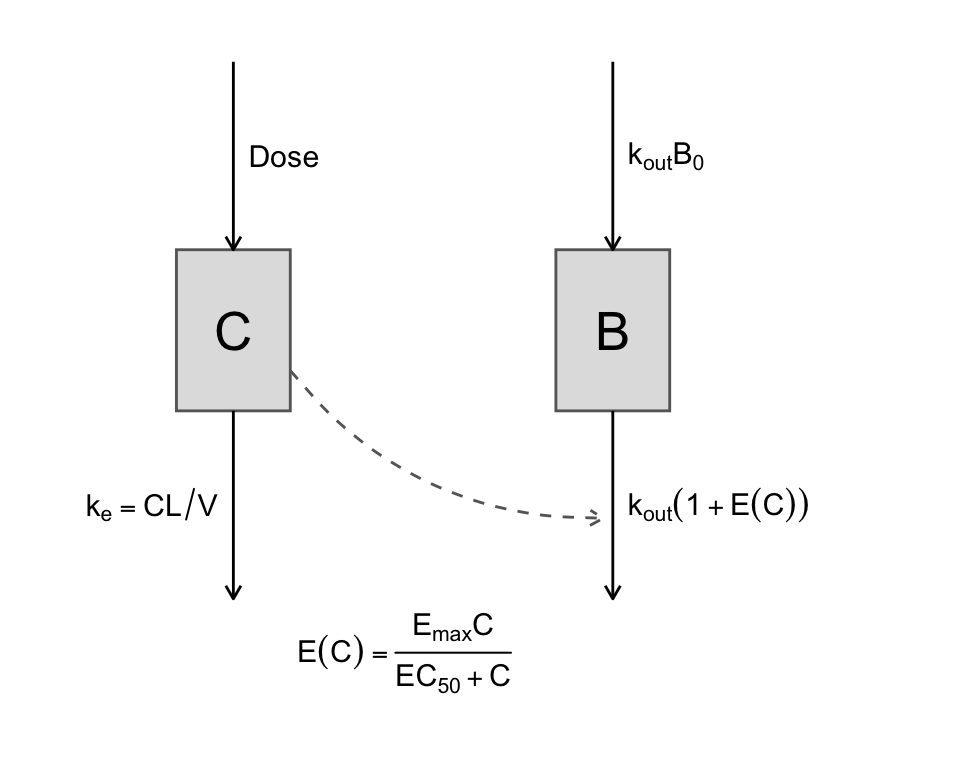
  • Monoclonal antibodies that deplete B cells are modelled with an indirect response: the drug raises the B-cell loss rate through \(E_{\max} C / (EC_{50} + C)\).
  • Published fits report \(E_{\max}\) near 150, and then do one of three things with \(EC_{50}\):
    • report it with a wide interval (paediatric rituximab: 13-fold CI)
    • fix it from in vitro binding (ofatumumab’s \(K_D\), rituximab in membranous nephropathy)
    • give up on it and fit a slope (inebilizumab: “less than the assay lower limit of quantitation”)

Is \(EC_{50}\) estimable at all, and if so, from what?

The answer

⚠️ \(EC_{50}\) is estimable only through \(E_{\max}\), and \(E_{\max}\) only from the first days of depletion, or from a cohort held in a narrow concentration band far below \(EC_{50}\).

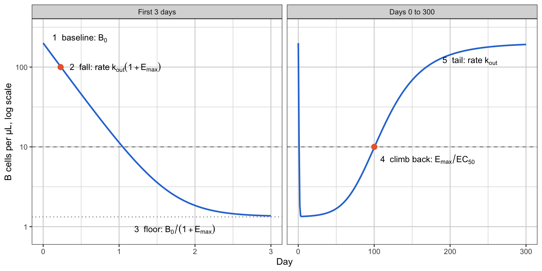
  • Each part of the B-cell curve carries one parameter or one combination:
    • the tail carries \(k_{\rm out}\)
    • the fall carries \(k_{\rm out}(1 + E_{\max})\)
    • the climb back carries the ratio \(S_0 = E_{\max}/EC_{50}\)
  • With a first sample at a week and doses that deplete below the limit, the fall is gone, and \(E_{\max}\) and \(EC_{50}\) are identified only as their ratio.
  • Fit the slope \(S_0\) unless a study samples the first days.

Out of scope

  • ❌ Target-mediated drug disposition. The PK here is linear.
  • ❌ Tissue B cells. Only the circulating count is modelled, because only it is measured.
  • ❌ A dose recommendation for any named drug. The published compounds are sources of parameter values and of what happened when the model was fit.

The model

Indirect response, drug stimulates loss

\[ \frac{dB}{dt} = k_{\rm out} B_0 - k_{\rm out}\big(1 + E(C)\big) B \]

\[ E(C) = \frac{E_{\max} C}{EC_{50} + C} \]

\[ C(t) = \frac{D}{V} e^{-k_e t} \]

  • Jusko’s type IV indirect response (Dayneka, Garg and Jusko 1993)
  • One-compartment PK, intravenous bolus
  • Only \(C/EC_{50}\) enters, so dose and \(EC_{50}\) scale together

Parameter values

Symbol What it is Value Why
\(B_0\) Baseline B-cell count 200 cells/µL Ofatumumab model 194, inebilizumab 135
\(k_{\rm out}\) B-cell loss rate 0.02 per day Half-life 35 d; ofatumumab 0.0124/d
\(E_{\max}\) Maximum fold-increase in loss 150 Ofatumumab 159, paediatric rituximab 155
\(EC_{50}\) Concentration for half of \(E_{\max}\) 1 mg/L Arbitrary scale
\(V\), \(CL\) Volume, clearance 3 L, 0.2 L/day Half-life 10.4 d, an IgG1
LOQ Flow-cytometry limit 5 or 10 cells/µL 2.5% or 5% of baseline
\(\sigma\) Proportional residual error 30% Inebilizumab model 61%

Published values are transcribed from the papers and not yet checked by eye.

Which part of the curve carries which parameter

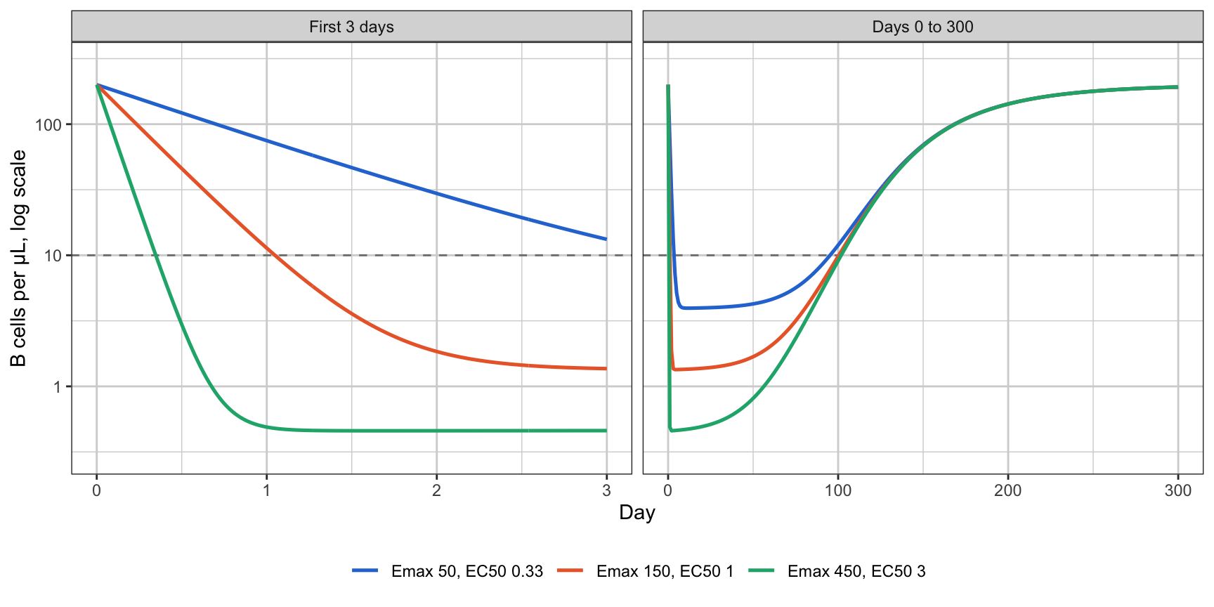
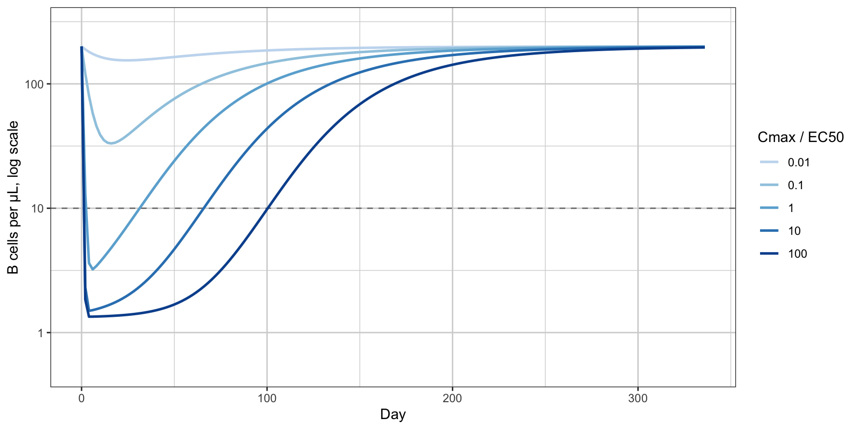
Five parts of the curve

Single dose with \(C_{\max} = 100 \times EC_{50}\). Dashed line: limit of quantification at 5% of baseline.

Two rates decide the shape

\[ \frac{d \ln B}{dt} = k_{\rm out} \left( \frac{B_0}{B} - 1 - E(C) \right) \]

  • \(B\) is pulled toward \(B_{\rm qss} = B_0 / (1 + E(C))\) at rate \(k_{\rm out}(1 + E(C))\).
  • The drug falls at rate \(k_e\).
\(k_{\rm out}(1+E)\) Compared with \(k_e = 0.067\)/day So \(B\)
Start, \(E = E_{\max}\) 3.0 per day 45 times faster follows the drug
End, \(E = 0\) 0.02 per day 0.3 times as fast lags, returns at its own pace

The curve starts fast and ends slow, so its parts separate.

The fall carries \(k_{\rm out}(1 + E_{\max})\)

For \(t \ll 1/k_e\) the concentration is still near \(C_{\max}\), so the equation is linear with constant coefficient:

\[ B(t) = B_{\rm ss} + (B_0 - B_{\rm ss})\, e^{-k_f t}, \qquad k_f = k_{\rm out}\big(1 + E(C_{\max})\big) \]

\[ t_{1/2,\rm fall} \approx \frac{\ln 2}{k_{\rm out}(1 + E_{\max})} \quad \text{for } C_{\max} \gg EC_{50} \]

  • Here: 0.23 days, five and a half hours. Over by day 1.5.
  • \(EC_{50}\) enters only through \(E(C_{\max}) = E_{\max}/(1 + EC_{50}/C_{\max})\), a 1% correction at \(C_{\max} = 100 \times EC_{50}\).
  • This is the only place \(E_{\max}\) appears without \(EC_{50}\) beside it, and it is over before a weekly sample arrives.
  • Published: the large-dose initial slope \(-k_{\rm out} B_0 E_{\max}\) (Sharma and Jusko 1996), and the fall curve as a lower bound at every dose that the response converges to (Peletier, Gabrielsson and Haag 2005).

The floor carries \(E_{\max}\), below the limit

After the fall, \(B\) tracks the quasi-steady state:

\[ B(t) \approx \frac{B_0}{1 + E\big(C(t)\big)} \approx \frac{B_0}{1 + E_{\max}} \quad \text{while } C \gg EC_{50} \]

  • Here: 1.3 cells/µL. The large-dose nadir of Sharma and Jusko 1996.
  • Above a limit at fraction \(f\) of baseline only if \(E_{\max} < 1/f - 1\): below 19 for a 5% limit, below 39 for 2.5%.
  • The two published models that estimate \(E_{\max}\) put it near 155, so the floor is censored.

The climb back carries \(E_{\max}/EC_{50}\)

The count crosses \(f B_0\) when \(E(C) = (1 - f)/f\). With \(C = C_{\max} e^{-k_e t}\):

\[ t_f = \underbrace{\frac{1}{k_e} \ln \frac{f\, S_0\, C_{\max}}{1 - f}}_{S_0 \text{ only}} + \underbrace{\frac{1}{k_e} \ln\left(1 - \frac{1 - f}{f E_{\max}}\right)}_{E_{\max} \text{ alone}} \]

  • The second term is all the separate information on \(E_{\max}\) that the recovery holds.
  • At \(f = 0.05\): \(-2.0\) days for \(E_{\max} = 150\), \(-7.2\) days for 50, \(-0.6\) days for 450.
  • A few days on a crossing near day 100, read through 30% error from monthly samples.

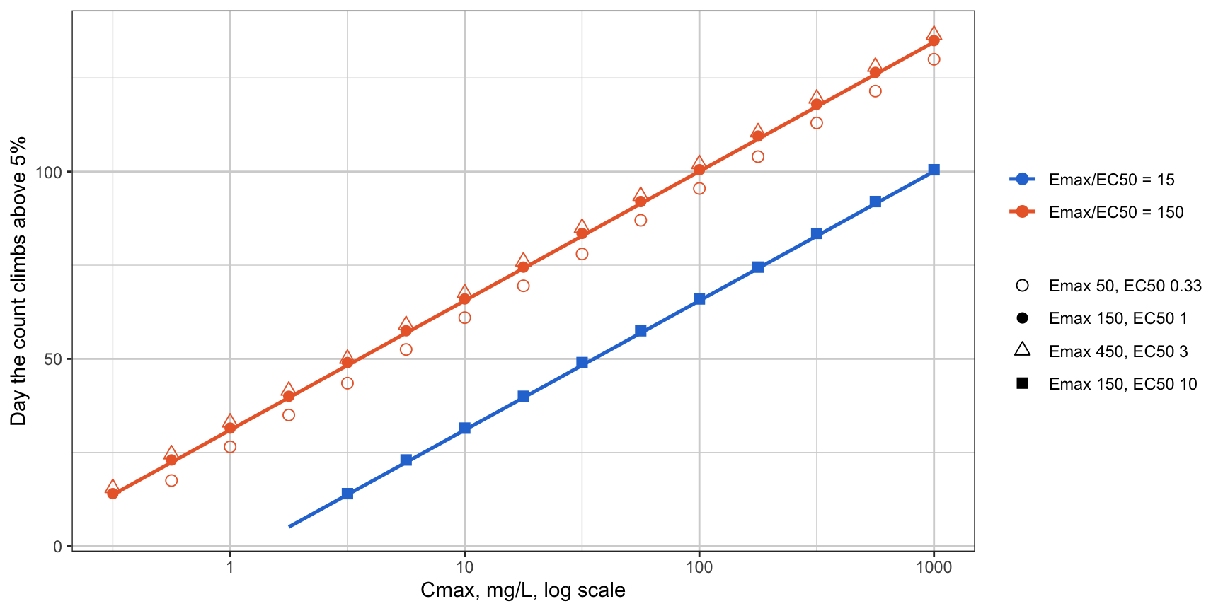
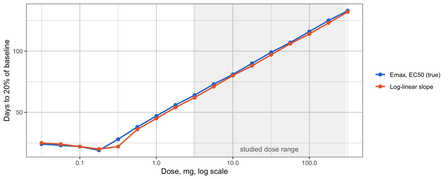
Across doses: Levy’s dose-duration line

  • Slope \(1/k_e\): each ten-fold dose adds \(\ln 10/k_e = 34.5\) days, 3.3 PK half-lives, whatever \(E_{\max}\) and \(EC_{50}\) are.
  • Three sets with the same ratio fall on one line. Levy (1966, as cited in secondary sources) gave this line for direct effects; the quasi-steady state makes it hold here.
  • Peletier et al. (2005) prove the general form: at large doses the recovery is a fixed shape travelling by \(\ln(C_{\max}/EC_{50})/k_e\).

The tail carries \(k_{\rm out}\); low doses carry \(S_0\)

Tail. Once \(S_0 C \ll 1\), the model is \(dB/dt = k_{\rm out}(B_0 - B)\):

\[ B_0 - B(t) \propto e^{-k_{\rm out} t} \qquad \text{(needs } k_{\rm out} < k_e\text{)} \]

Doses that stay below \(EC_{50}\). \(E(C) \approx S_0 C\) for the whole curve, so the model holds \(E_{\max}\) and \(EC_{50}\) only as their ratio. For shallow depletion:

\[ \varepsilon_{\max} = 1 - \frac{B_{\min}}{B_0} = S_0 C_{\max} \left(\frac{k_{\rm out}}{k_e}\right)^{k_e/(k_e - k_{\rm out})} \]

  • A low-dose cohort informs the slope, not its two factors.

The area between curves follows \(S_0\) too

\[ \text{area} = \int_0^\infty (B_0 - B)\,dt \;\sim\; \frac{B_0}{k_e} \frac{E_{\max}}{1 + E_{\max}} \ln\left(1 + \frac{C_{\max}}{EC_{50}}\right) \quad \text{(large dose)} \]

Cmax Emax EC50 Area, ODE Large-dose formula
1 50 0.33 21407 4077
1 150 1.00 21715 2066
1 450 3.00 21818 861
100 50 0.33 34999 16786
100 150 1.00 35481 13754
100 450 3.00 35631 10585
  • Sharma and Jusko (1996) and Peletier et al. (2005): read \(E_{\max}\) from the slope of area against log dose. At \(E_{\max} = 150\) the slope factor is 0.993, so the slope carries almost nothing.
  • At a given dose the area is the same for all three sets: it follows \(S_0\). The formula’s level is low because its omitted constant is large here.

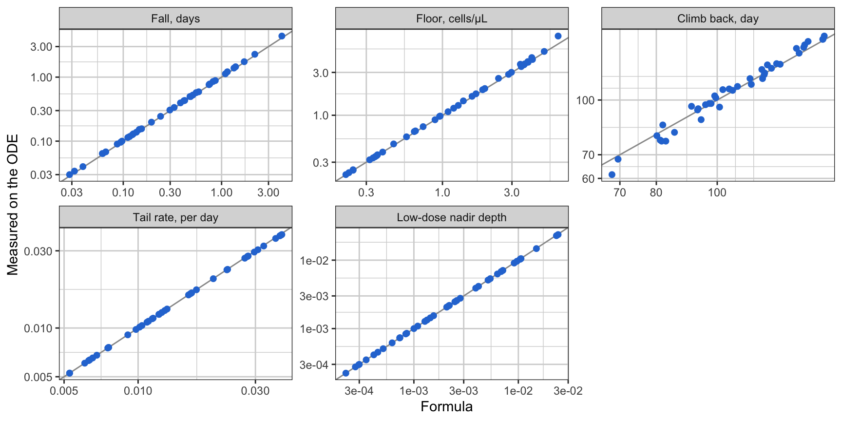
Each formula against the ODE solution

Forty random parameter sets: \(E_{\max}\) 30 to 1000, \(EC_{50}\) 0.1 to 10, \(k_{\rm out}\) 0.005 to 0.04 per day. Largest misses are where \(C_{\max}\) is only 30 × \(EC_{50}\) or \(k_{\rm out}\) is small.

What is identifiable and what is not

Part of the curve Carries Observed when Usual B-cell study
Baseline \(B_0\) always ✅
Fall \(k_{\rm out}(1 + E_{\max})\) samples in the first one to two days ❌ first sample at a week
Floor \(E_{\max}\) \(E_{\max} < 1/f - 1\) ❌ below the limit
Climb back \(S_0\), plus a few-day \(E_{\max}\) term samples through recovery, PK known ✅
Tail \(k_{\rm out}\) samples until repopulation ✅
Low-dose cohort \(S_0\), \(k_{\rm out}\) \(C_{\max} \ll EC_{50}\) ✅ but adds no \(E_{\max}\)
  • ✅ Always: \(B_0\), \(k_{\rm out}\), \(S_0 = E_{\max}/EC_{50}\)
  • ⚠️ \(E_{\max}\): only from the fall, or a floor above the limit
  • ❌ \(EC_{50}\) alone: from no part of the curve; identified exactly when \(E_{\max}\) is

The model is structurally identifiable. The loss is practical, caused by the quantification limit and the sampling schedule.

The textbook recipe needs the two readings a study loses

Sharma and Jusko (1998), Table 1, recover the parameters graphically:

  1. Baseline → \(B_0\)
  2. Large-dose nadir → \(E_{\max} = B_0/B_{\min} - 1\)
  3. Initial slope with \(E_{\max}\) → \(k_{\rm in}\), then \(k_{\rm out} = k_{\rm in}/B_0\)
  4. Concentration at the time of the nadir → \(EC_{50}\)

Design: two or more bolus doses, one high enough for full effect, and the baseline.

  • ❌ Step 2: the nadir is 1.3 cells/µL, below the limit.
  • ❌ Step 3: the initial slope is over in a day, before a weekly sample.
  • What is left is the tail, for \(k_{\rm out}\), and the climb back, for \(E_{\max}/EC_{50}\).

Same ratio, same curve above the limit

Three-fold differences in \(E_{\max}\) and \(EC_{50}\) at fixed ratio. Above the limit the curves differ in the first two days and nowhere else.
Why a large Emax makes it worse

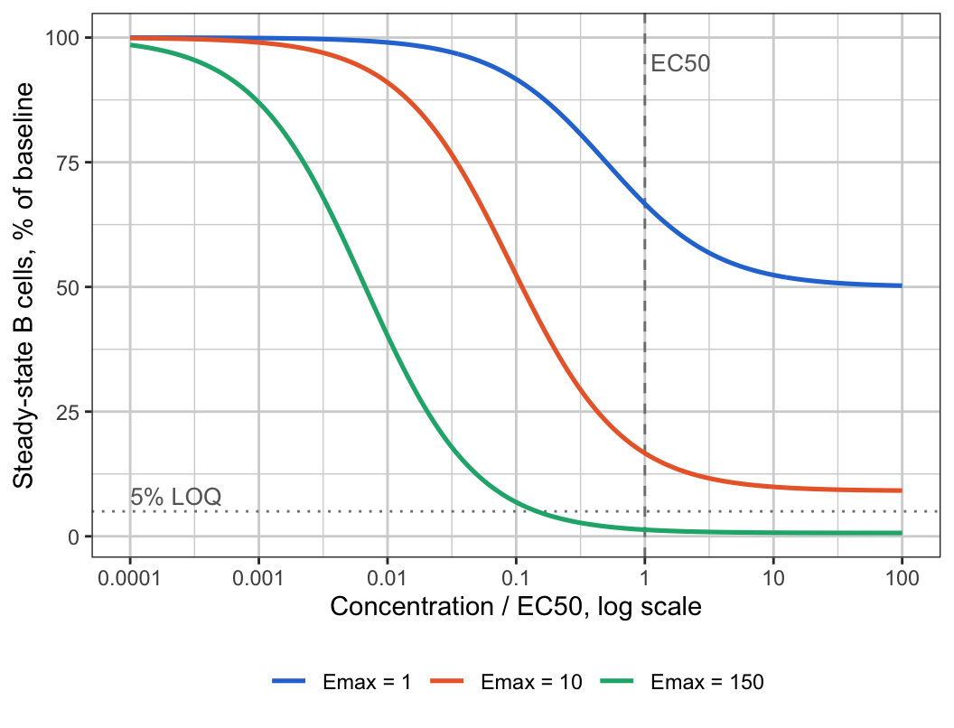
Half-maximal depletion is far below EC50

\[ \frac{B_{ss}}{B_0} = \frac{1}{1 + E(C)} \]

Half of baseline needs \(E = 1\):

\[ C_{1/2} = \frac{EC_{50}}{E_{\max} - 1} \]

  • \(E_{\max} = 150\): \(C_{1/2} = EC_{50}/149\)
  • At \(C = EC_{50}\) the count is already 1.3% of baseline
  • The quantifiable band is about \(EC_{50}/1500\) to \(EC_{50}/15\), below every therapeutic dose
  • Krzyzanski and Jusko (1998): two infusion rates give \(E_{\max}\) and \(EC_{50}\) only if both concentrations are not well above \(EC_{50}\)

What a study sees

Five single doses a ten-fold apart

  • From 1 to 100 × \(EC_{50}\): same fall, same floor, all below the limit for two months. Only the start of recovery differs, by 34.5 days per ten-fold.
  • The only curve quantifiable throughout is at 0.01 × \(EC_{50}\), in the linear range, where it carries \(S_0\).

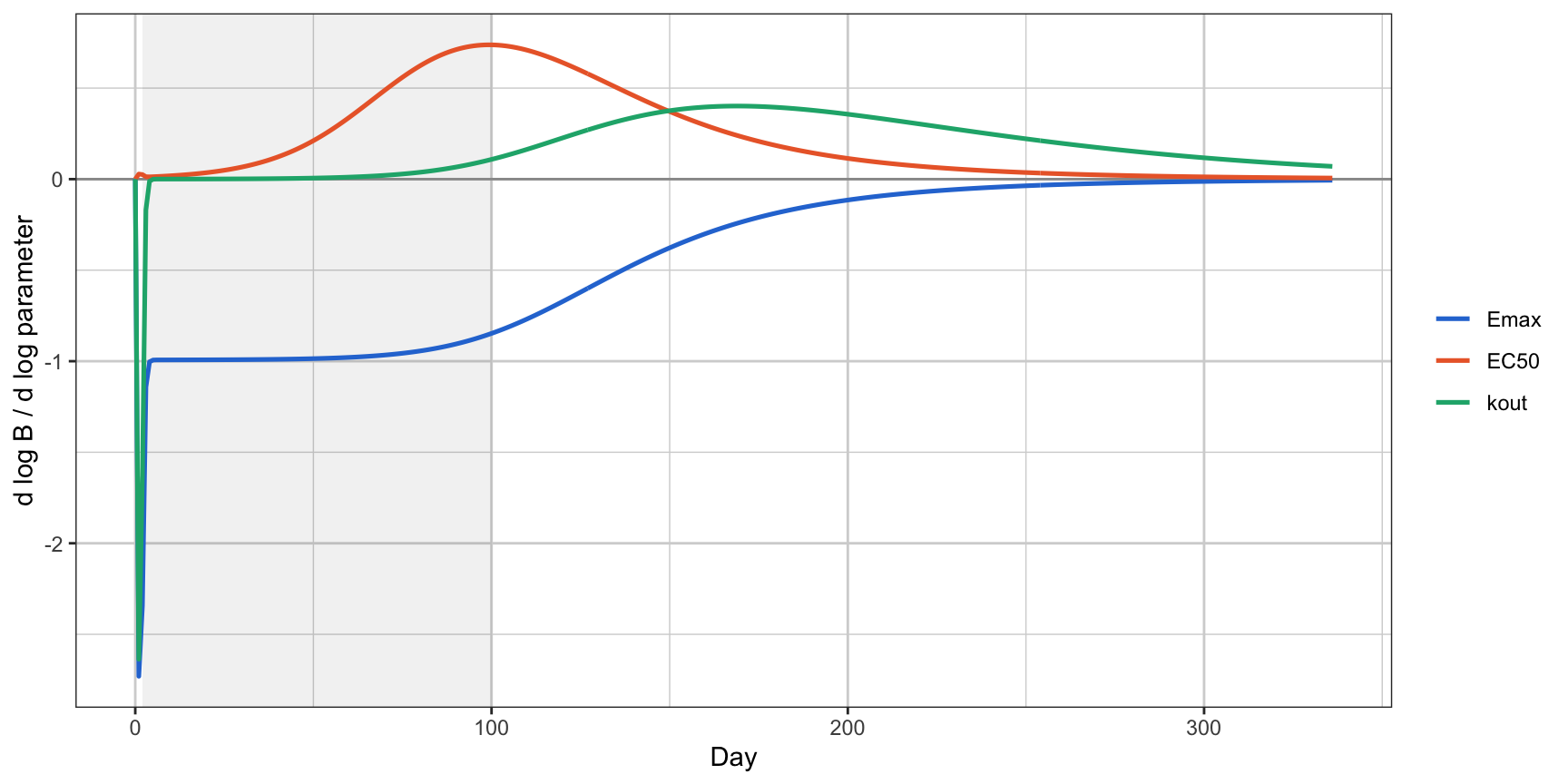
Where the information lives: sensitivities

  • Days 0 to 3: \(E_{\max}\) and \(k_{\rm out}\) equal, \(EC_{50}\) near zero.
  • Days 4 to 80 (shaded): below the limit, no information.
  • Days 80 to 200: \(E_{\max}\) and \(EC_{50}\) equal and opposite: only the ratio. \(k_{\rm out}\) is last standing in the tail.

Expected precision by design

Design First sample RSE Emax % RSE EC50 % corr(Emax, EC50) RSE Emax/EC50 % RSE k_out %
A: 300 mg, 6 patients Day 1 41 55 0.94 21 39
B: 30, 100, 300 mg; 4 each Day 1 26 34 0.94 13 24
C: 3 to 300 mg, five levels; 4 each Day 1 12 13 0.83 7 10
D: C with 0.03, 0.3 mg for 10, 100 Day 1 10 9 0.72 7 8
A: 300 mg, 6 patients Day 7 833 894 1.00 65 56
B: 30, 100, 300 mg; 4 each Day 7 127 144 1.00 21 28
C: 3 to 300 mg, five levels; 4 each Day 7 109 123 1.00 17 20
D: C with 0.03, 0.3 mg for 10, 100 Day 7 90 98 1.00 11 9

Fisher information, LOQ 5 cells/µL, 30% proportional error, observations below the limit dropped.

  • The slope and \(k_{\rm out}\) are estimated in every design.
  • \(E_{\max}\) and \(EC_{50}\) need days 1 and 3. Without them, correlation 1.00 in every design, including D with its low-dose cohorts.

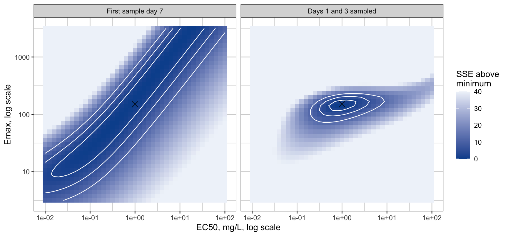
The likelihood ridge

  • Left: a ridge along \(E_{\max}/EC_{50}\) = constant. Any point on it fits equally well.
  • Right: the fall closes it to a basin around the truth (cross).
  • Dutta, Matsumoto and Ebling (1996): good fit, precise descriptors inside the data, wrong \(E_{\max}\) and \(EC_{50}\).

The published record

Five published B-cell depletion models

Drug Data What happened to \(EC_{50}\)
Ofatumumab 1,486 patients, 3 to 700 mg, partial-depletion arms at 3 and 10 mg SC ✅ Estimated, RSE 8.5%; \(E_{\max}\) 159
Rituximab, paediatric 63 patients, full dose, 52% of counts below limit ⚠️ \(ED_{50}\) RSE 61%, CI 0.18 to 2.26 mg
Inebilizumab 213 subjects, 100-fold dose range ❌ Abandoned for a log-linear slope
Rituximab, membranous nephropathy 41 patients ❌ None; TMDD binding constant at 60% RSE
Ianalumab Phase 2 and RA data ❌ Not reported; receptor-occupancy model added
  • Ofatumumab had cohorts in the band and subcutaneous absorption that slowed the fall into the sampling window.
  • Paediatric rituximab is the ridge. Inebilizumab is the ridge recognized.

Values transcribed from the papers by a fetch tool, not yet checked by eye.

What to do

Fit the slope

Schoemaker, van Gerven and Cohen (1998): when the data do not approach \(E_{\max}\), report \(S_0 = E_{\max}/EC_{50}\).

The duration of depletion depends on \(S_0\) and \(k_{\rm out}\), so a slope model loses nothing inside the studied dose range.

What a study needs if it wants EC50

In the order they would be dropped from a protocol:

  1. B-cell samples on days 1 and 3 after the first dose. The only observation that separates \(E_{\max}\) from \(EC_{50}\) at a therapeutic dose.
  2. B cells monthly until repopulation. The tail gives \(k_{\rm out}\), and without it the fall gives nothing.
  3. A PK assay below \(EC_{50}/E_{\max}\), or an explicit extrapolation of the PK tail.
  4. A cohort whose nadir is quantifiable and sits in the band, if the design can afford one. Below the band informs the slope only.
  5. Failing 1 and 4, fit the slope, report \(S_0\) with its interval, and fix one factor from in vitro binding if the factors are needed.

For the ITP project

  • The ITP dose escalation: three to six patients per level, first B-cell sample at a week.
  • That design identifies the slope and \(k_{\rm out}\), and neither \(E_{\max}\) nor \(EC_{50}\).
  • Parameterizing by the slope is right.
  • Adding days 1 and 3 makes the \(E_{\max}\) form fittable at about 10% RSE across five cohorts, for two extra blood draws.

Open questions

  • Sigmoidicity. A Hill coefficient above 1 sharpens the band. Is it identifiable alongside the slope?
  • Subcutaneous dosing. Absorption slows the fall into the first week, which may be how the ofatumumab model saw it.
  • Censoring. A likelihood with censored terms would recover some information at the floor.
  • Between-patient variability. The precision numbers are for fixed parameters and are optimistic.

References

  • Dayneka, Garg, Jusko 1993. J Pharmacokinet Biopharm 21:457. The four indirect-response models.
  • Levy 1966. Clin Pharmacol Ther 7:362. Duration of effect linear in log dose. Not obtained; cited from secondary sources.
  • Sharma, Jusko 1996. J Pharmacokinet Biopharm 24:611. Dose and \(EC_{50}\) scale together.
  • Krzyzanski, Jusko 1997. J Pharmacokinet Biopharm 25:107. Mathematical properties of the four models. Not obtained; its large-dose limits are cited as given in Sharma and Jusko 1996.
  • Peletier, Gabrielsson, Haag 2005. J Pharmacokinet Pharmacodyn 32:607. Dynamical systems analysis of the indirect response model.
  • Sharma, Jusko 1998. Br J Clin Pharmacol 45:229. Review; Table 1 is the graphical identification recipe.
  • Krzyzanski, Jusko 1998. J Pharmacokinet Biopharm 26:385. The four models under infusion.
  • Dutta, Matsumoto, Ebling 1996. J Pharm Sci 85:232. \(E_{\max}\) from truncated data.
  • Schoemaker, van Gerven, Cohen 1998. J Pharmacokinet Biopharm 26:581. Potency without the maximum: the slope \(S_0\).
  • Janzén et al. 2016. Front Physiol 7:590. Structural identifiability of pharmacodynamic models.

Full list with status markers: references. Working document: EC50 identifiability.