flowchart LR
    A["Recovery tail<br/>days 150 to 300"] --> K["k_out"]
    B["Speed of the fall<br/>days 0 to 3"] --> KE["k_out × Emax"]
    C["When recovery starts<br/>days 80 to 140"] --> R["Emax / EC50"]
    K --> KE
    KE --> E["Emax"]
    E --> R
    R --> EC["EC50"]
Why EC50 is hard to estimate for a B-cell depleting agent
Where the information about Emax and EC50 lives in an indirect-response model, and what a study has to contain to see it
pharmacometrics
identifiability
immunology
working document
For a drug that depletes circulating B cells through an indirect-response model, the Emax and EC50 of the drug effect are separately identifiable only from the first days of depletion and from cohorts sitting in a narrow concentration band far below therapeutic exposure. This document derives that, simulates it, and checks it against the published models.
The simulations here run on every render and the published numbers do not. Everything computed on this page comes from the code chunks in it, with parameter values chosen to resemble published models and stated where they are chosen. The published estimates in Section 7 were transcribed from the papers by a fetch tool and carry ⚠️ in references.qmd; the theory sources are from abstracts and carry ❌. The project index lists the other documents in this folder. This project grew out of Section 6.2 of the ITP-PK-Platelet specification.
In brief
The question. A monoclonal antibody depletes circulating B cells. The standard model is an indirect response with the drug raising the B-cell loss rate through \(E_{\max} C / (EC_{50} + C)\). Published fits of this model report \(E_{\max}\) near 150, and either report \(EC_{50}\) with a wide interval, or fix it, or give up on it and fit a slope instead. Is \(EC_{50}\) estimable at all, and if so from what?
The answer. ⚠️ \(EC_{50}\) is estimable only through \(E_{\max}\), and \(E_{\max}\) is estimable only from the first days of depletion or from a cohort held in a concentration band two orders of magnitude below \(EC_{50}\). With a first post-dose B-cell sample at a week and doses that deplete completely, the two parameters are perfectly correlated and only their ratio is identified. Three quantities in the data carry three pieces of information: the recovery tail carries \(k_{\rm out}\); the speed of the initial fall carries \(k_{\rm out} E_{\max}\); the timing of the recovery’s start carries \(E_{\max}/EC_{50}\). Lose the first days, and the second piece is gone, and \(E_{\max}\) and \(EC_{50}\) collapse onto one ridge. This is Section 4, and Section 5 puts numbers on it by design.
Why a large \(E_{\max}\) makes it worse. The nadir is \(B_0/(1 + E)\). With \(E_{\max} = 150\), the count at \(C = EC_{50}\) is already 1.3% of baseline, below any flow-cytometry limit. Half-maximal depletion happens at \(C \approx EC_{50}/150\). The concentration band over which the cell count can say anything about \(EC_{50}\) separately from \(E_{\max}\) is therefore far below every therapeutic dose, and usually below the PK assay. Section 3.
What to do instead. Parameterize the drug effect as the slope \(S_0 = E_{\max}/EC_{50}\), which is what Schoemaker et al. proposed in 1998 for exactly this situation and what the inebilizumab model did in 2022, and test the \(E_{\max}\) form only when a cohort has a quantifiable nadir. Section 8. Everything downstream that depends on the duration of depletion depends on the slope and \(k_{\rm out}\), and loses nothing.
Out of scope, stated once.
- ❌ Target-mediated drug disposition. The PK here is linear. Where a published model ties the effect to receptor occupancy with a binding constant fixed from in vitro data, that is a different route to the same place and Section 7 notes it.
- ❌ Tissue B cells. Only the circulating count is modelled, because only it is measured.
- ❌ Any recommendation about a named drug’s dose. The compounds in Section 7 are sources of parameter values and of what happened when the model was fit.
1. The model
An indirect response model of the fourth Jusko type: the drug stimulates the loss of the response variable. With \(B\) the circulating B-cell count,
\[ \frac{dB}{dt} = k_{\rm in} - k_{\rm out}\,\big(1 + E(C)\big)\,B, \qquad E(C) = \frac{E_{\max}\, C}{EC_{50} + C}, \qquad B(0) = B_0 = \frac{k_{\rm in}}{k_{\rm out}} \]
and one-compartment PK after an intravenous bolus, \(C(t) = (D/V) e^{-k_e t}\).
| Symbol | What it is | Value used here | Why that value |
|---|---|---|---|
| \(B_0\) | Baseline B-cell count | 200 cells/µL | Typical adult; ofatumumab model 194, inebilizumab 135 |
| \(k_{\rm out}\) | B-cell loss rate; sets the repopulation speed | 0.02 per day | Half-life 35 d; ofatumumab 0.0124/d, paediatric rituximab CD19 half-life 173 d |
| \(E_{\max}\) | Maximum fold-increase in loss rate | 150 | Ofatumumab 159, paediatric rituximab 155 |
| \(EC_{50}\) | Concentration for half of \(E_{\max}\) | 1 mg/L | Arbitrary scale; only \(C/EC_{50}\) enters |
| \(V\), \(CL\) | Volume, clearance | 3 L, 0.2 L/day | Half-life 10.4 d, an IgG1 antibody |
| LOQ | Flow-cytometry limit for B cells | 5 or 10 cells/µL | 2.5% or 5% of baseline |
| \(\sigma\) | Proportional residual error | 30% | Inebilizumab model 61%, ofatumumab lower; 30% is generous to the design |
The published values are in references.qmd, entries 5 to 8, transcribed and not verified.
library(ggplot2); library(dplyr); library(tidyr); library(xgxr)
set.seed(20260909); xgx_theme_set()
knitr::opts_chunk$set(fig.height = 4, fig.width = 6.5)
# Palette: the first three categorical slots of the reference palette in the
# dataviz skill, documented as validated for all pairs; a single-hue ramp for dose.
pal3 <- c("#2a78d6", "#eb6834", "#1baf7a")
ramp5 <- c("#c6dbef", "#9ecae1", "#6baed6", "#3182bd", "#08519c")

Emax <- 150; EC50 <- 1; kout <- 0.02; B0 <- 200; V <- 3; CL <- 0.2

sim_B <- function(dose, Emax, EC50, kout, B0 = 200, times, dt = 0.1,
                  form = "emax", S = NA, Cref = NA) {
  ke <- CL / V
  Cfun <- function(t) dose / V * exp(-ke * t)
  eff <- if (form == "emax") function(C) Emax * C / (EC50 + C) else function(C) S * log1p(C / Cref)
  # Exponential integrator: within each step the concentration is held at its
  # midpoint value, so dB/dt = a - b B has the exact solution below. It is
  # stable for any b * dt, which RK4 is not when Emax is in the thousands.
  tgrid <- seq(0, max(times), by = dt); res <- numeric(length(tgrid)); B <- B0; res[1] <- B
  a <- kout * B0
  for (i in 2:length(tgrid)) {
    b <- kout * (1 + eff(Cfun(tgrid[i - 1] + dt / 2)))
    B <- a / b + (B - a / b) * exp(-b * dt); res[i] <- B
  }
  approx(tgrid, res, xout = times)$y
}
2. What the data look like
Five single doses a ten-fold apart, the highest giving a peak concentration of 100 × \(EC_{50}\) and the lowest 0.01 × \(EC_{50}\). The horizontal line is a flow-cytometry limit of 10 cells/µL.
tt <- seq(0, 336, by = 2)
doses <- c(0.03, 0.3, 3, 30, 300)
prof <- bind_rows(lapply(doses, function(d)
  data.frame(dose = d, cmax = d / V, day = tt, B = sim_B(d, Emax, EC50, kout, B0, times = tt))))
prof$label <- factor(sprintf("%g", prof$cmax), levels = sprintf("%g", doses / V))
ggplot(prof, aes(day, B, colour = label)) +
  geom_hline(yintercept = 10, linetype = 2, colour = "grey50") +
  geom_line(linewidth = 0.8) +
  scale_colour_manual(values = ramp5, name = "Cmax, multiples of EC50") +
  scale_y_log10(breaks = c(1, 10, 100), limits = c(0.5, 300)) +
  annotate("text", x = 330, y = 10, label = "LOQ", hjust = 1, vjust = -0.4, size = 3, colour = "grey40") +
  labs(x = "Day", y = "B cells per µL, log scale") +
  theme(legend.position = "bottom")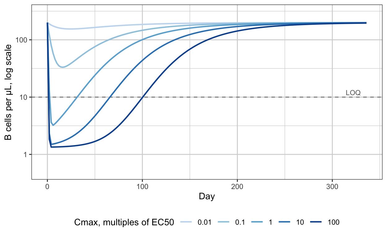
Two things to read off. Between \(C_{\max} = 1 \times EC_{50}\) and \(100 \times EC_{50}\) the curves are indistinguishable for the first two months: same fall, same floor, all below the limit. What differs is when recovery starts, and it starts later by about one PK half-life for each ten-fold increase in dose. And the only curve that stays quantifiable throughout is the lowest, at \(C_{\max} = 0.01 \times EC_{50}\), where the drug effect is in its linear range and says nothing about \(EC_{50}\) on its own.
3. The arithmetic of a large Emax
At a steady concentration \(C\), the count settles at
\[ \frac{B_{ss}}{B_0} = \frac{1}{1 + E(C)} = \frac{1}{1 + E_{\max} C/(EC_{50} + C)} \]
so that half-maximal depletion, \(B_{ss} = B_0/2\), needs \(E = 1\), which is at
\[ C_{1/2} = \frac{EC_{50}}{E_{\max} - 1} \]
For \(E_{\max} = 150\) that is \(EC_{50}/149\). The concentration that halves the drug’s effect on the rate and the concentration that halves the cell count are two orders of magnitude apart.
cc <- 10^seq(-4, 2, length.out = 300)
dep <- bind_rows(lapply(c(1, 10, 150), function(em)
  data.frame(Emax = em, C = cc, frac = 1 / (1 + em * cc / (1 + cc)))))
dep$Emax <- factor(paste("Emax =", dep$Emax), levels = paste("Emax =", c(1, 10, 150)))
ggplot(dep, aes(C, 100 * frac, colour = Emax)) +
  geom_vline(xintercept = 1, linetype = 2, colour = "grey50") +
  geom_hline(yintercept = 5, linetype = 3, colour = "grey50") +
  geom_line(linewidth = 0.8) +
  scale_colour_manual(values = pal3, name = NULL) +
  scale_x_log10(breaks = 10^(-4:2), labels = c("0.0001", "0.001", "0.01", "0.1", "1", "10", "100")) +
  annotate("text", x = 1, y = 95, label = "EC50", hjust = -0.1, size = 3, colour = "grey40") +
  annotate("text", x = 1e-4, y = 5, label = "5% LOQ", hjust = 0, vjust = -0.4, size = 3, colour = "grey40") +
  labs(x = "Concentration, multiples of EC50, log scale", y = "Steady-state B cells, % of baseline") +
  theme(legend.position = "bottom")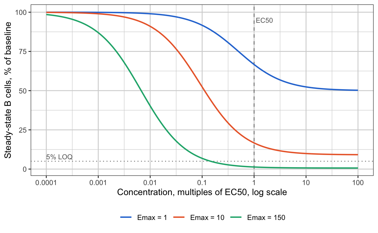
The consequence is a band. Below \(C_{1/2}/10\) the effect is small and linear in \(C\) with slope \(E_{\max}/EC_{50}\). Above \(EC_{50}\) the count is below the limit whatever \(C\) is. In between, the count is quantifiable and its level depends on \(E_{\max}\) and \(EC_{50}\) separately. That band, roughly \(EC_{50}/1500\) to \(EC_{50}/15\) here, is where a cohort would have to sit for the nadir to identify the two parameters, and no therapeutic dose sits there.
4. Where the information lives
The sensitivity of the log count to each log parameter, along the top-dose profile, says what each observation can tell the estimator.
tt <- seq(0, 336, by = 1); h <- 1e-4
f0 <- sim_B(300, Emax, EC50, kout, B0, times = tt)
sens <- data.frame(day = tt,
  Emax = (log(sim_B(300, Emax * exp(h), EC50, kout, B0, times = tt)) - log(f0)) / h,
  EC50 = (log(sim_B(300, Emax, EC50 * exp(h), kout, B0, times = tt)) - log(f0)) / h,
  kout = (log(sim_B(300, Emax, EC50, kout * exp(h), B0, times = tt)) - log(f0)) / h,
  B = f0)
blq <- range(sens$day[sens$B < 0.05 * B0])
sl <- pivot_longer(sens, c(Emax, EC50, kout), names_to = "parameter", values_to = "s")
sl$parameter <- factor(sl$parameter, levels = c("Emax", "EC50", "kout"))
ggplot(sl, aes(day, s, colour = parameter)) +
  annotate("rect", xmin = blq[1], xmax = blq[2], ymin = -Inf, ymax = Inf, alpha = 0.08, fill = "grey30") +
  geom_hline(yintercept = 0, colour = "grey60") +
  geom_line(linewidth = 0.8) +
  scale_colour_manual(values = pal3, name = NULL) +
  labs(x = "Day", y = "d log B / d log parameter") +
  theme(legend.position = "bottom")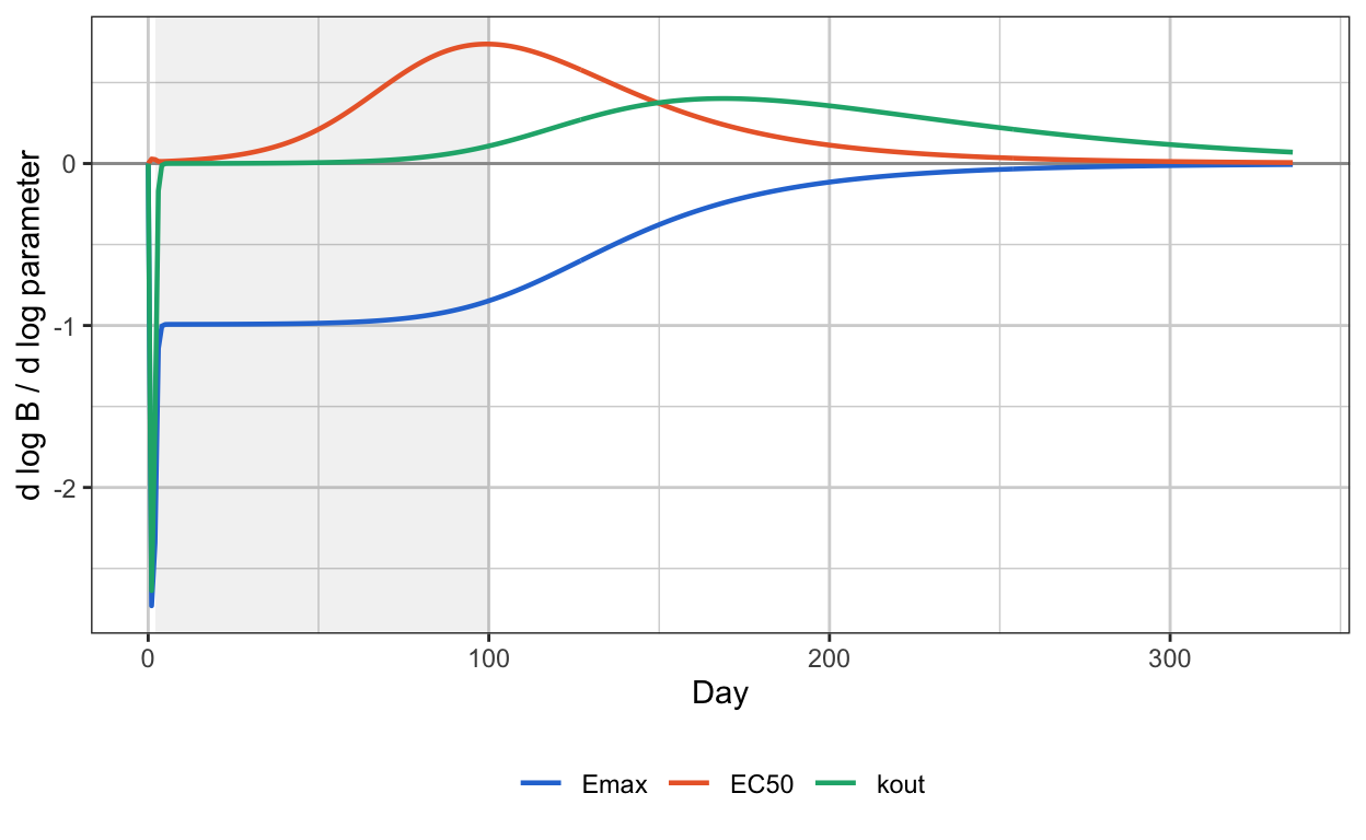
Three regions, and each one identifies one thing.
Days 0 to 3, the fall. Sensitivity to \(E_{\max}\) and to \(k_{\rm out}\) are both large and equal, and sensitivity to \(EC_{50}\) is near zero. At high concentration the loss rate is \(k_{\rm out}(1 + E_{\max})\), so the speed of the fall identifies the product \(k_{\rm out} E_{\max}\) and nothing about \(EC_{50}\). This is the only place \(E_{\max}\) appears without \(EC_{50}\) beside it.
Days 4 to 80, the floor. Everything is below the limit. No observations, no information.
Days 80 to 200, the recovery. Sensitivity to \(E_{\max}\) and \(EC_{50}\) are equal and opposite: raising one or lowering the other shifts the curve the same way. Recovery begins when \(E(C)\) falls to order 1, which happens at \(C \approx EC_{50}/E_{\max}\), so this region identifies the ratio and only the ratio. Sensitivity to \(k_{\rm out}\) rises through the recovery and is the last thing standing at day 250, so the tail identifies \(k_{\rm out}\) alone.
The chain in the In brief diagram follows. \(k_{\rm out}\) from the tail; \(k_{\rm out} E_{\max}\) from the fall, hence \(E_{\max}\); \(E_{\max}/EC_{50}\) from the recovery’s timing, hence \(EC_{50}\). Remove the fall from the data and the chain breaks at its second link.
5. Expected precision by design
The Fisher information for the four log-parameters, from the sensitivities at each sampling time, summed over patients and dose levels, with observations below the limit dropped. Dropping them understates the information slightly, since a censored value still says the count is below the limit, and the comparison between designs is unaffected. Four dose designs, two limits, and two sampling schedules that differ only in whether days 1 and 3 are sampled.
t_dense  <- c(0, 1, 3, 7, 14, 28, 56, 84, 112, 140, 168, 224, 280, 336)
t_sparse <- c(0, 7, 14, 28, 56, 84, 112, 140, 168, 224, 280, 336)
fim_design <- function(doses_n, loq, sigma = 0.3, times) {
  th <- log(c(Emax, EC50, kout, B0)); J <- NULL
  for (k in seq_along(doses_n$dose)) {
    d <- doses_n$dose[k]; n <- doses_n$n[k]
    f0 <- sim_B(d, Emax, EC50, kout, B0, times = times); keep <- f0 >= loq
    Jd <- sapply(1:4, function(j) { h <- 1e-4; th2 <- th; th2[j] <- th2[j] + h; p <- exp(th2)
      (log(sim_B(d, p[1], p[2], p[3], p[4], times = times)) - log(f0)) / h })
    J <- rbind(J, sqrt(n) * Jd[keep, , drop = FALSE])
  }
  Fi <- t(J) %*% J / sigma^2
  Vm <- tryCatch(solve(Fi), error = function(e) matrix(NA, 4, 4))
  se <- sqrt(diag(Vm))
  data.frame(rse_Emax = 100 * se[1], rse_EC50 = 100 * se[2],
             corr = Vm[1, 2] / sqrt(Vm[1, 1] * Vm[2, 2]),
             rse_slope = 100 * sqrt(Vm[1, 1] + Vm[2, 2] - 2 * Vm[1, 2]),
             rse_kout = 100 * se[3], n_obs = nrow(J))
}
designs <- list(
  "A: 300 mg only, 6 patients"                 = data.frame(dose = 300, n = 6),
  "B: 30, 100, 300 mg; 4 each"                 = data.frame(dose = c(30, 100, 300), n = 4),
  "C: 3 to 300 mg, five levels; 4 each"        = data.frame(dose = c(3, 10, 30, 100, 300), n = 4),
  "D: C with 0.03 and 0.3 mg replacing 10, 100" = data.frame(dose = c(0.03, 0.3, 3, 30, 300), n = 4))
grid <- expand.grid(design = names(designs), loq = c(5, 10), sampling = c("first sample day 1", "first sample day 7"),
                    stringsAsFactors = FALSE)
res <- bind_rows(lapply(seq_len(nrow(grid)), function(i) {
  tt <- if (grid$sampling[i] == "first sample day 1") t_dense else t_sparse
  cbind(grid[i, ], fim_design(designs[[grid$design[i]]], loq = grid$loq[i], times = tt))
}))
res %>% filter(loq == 5) %>% select(sampling, design, rse_Emax, rse_EC50, corr, rse_slope, rse_kout, n_obs) %>%
  arrange(sampling, design) %>%
  knitr::kable(digits = c(0, 0, 0, 0, 2, 0, 0, 0),
    col.names = c("Sampling", "Design", "RSE Emax %", "RSE EC50 %", "corr(Emax, EC50)", "RSE Emax/EC50 %", "RSE k_out %", "Observations kept"),
caption = "Expected precision from the Fisher information, LOQ 5 cells/µL (2.5% of baseline), 30% proportional error")| Sampling | Design | RSE Emax % | RSE EC50 % | corr(Emax, EC50) | RSE Emax/EC50 % | RSE k_out % | Observations kept |
|---|---|---|---|---|---|---|---|
| first sample day 1 | A: 300 mg only, 6 patients | 41 | 55 | 0.94 | 21 | 39 | 8 |
| first sample day 1 | B: 30, 100, 300 mg; 4 each | 26 | 34 | 0.94 | 13 | 24 | 27 |
| first sample day 1 | C: 3 to 300 mg, five levels; 4 each | 12 | 13 | 0.83 | 7 | 10 | 49 |
| first sample day 1 | D: C with 0.03 and 0.3 mg replacing 10, 100 | 10 | 9 | 0.72 | 7 | 8 | 58 |
| first sample day 7 | A: 300 mg only, 6 patients | 832 | 894 | 1.00 | 65 | 56 | 7 |
| first sample day 7 | B: 30, 100, 300 mg; 4 each | 127 | 144 | 1.00 | 21 | 28 | 24 |
| first sample day 7 | C: 3 to 300 mg, five levels; 4 each | 109 | 123 | 1.00 | 17 | 20 | 43 |
| first sample day 7 | D: C with 0.03 and 0.3 mg replacing 10, 100 | 90 | 98 | 1.00 | 11 | 9 | 50 |
Read down the right-hand columns first. The slope \(E_{\max}/EC_{50}\) and \(k_{\rm out}\) are estimated in every design, at a precision that improves with cohorts and does not depend much on the early samples. Then read \(E_{\max}\) and \(EC_{50}\) against the sampling column. With days 1 and 3 sampled they are estimable, at 40 to 55% RSE from six patients at one dose and around 10% from five cohorts. With the first sample at day 7 they are not estimable in any design: the correlation is 1.00 and the RSEs run from about 90% to over 800%. Design D, which puts two cohorts at concentrations where the nadir is quantifiable, does not rescue them, because those cohorts sit in the linear range below the band of Section 3 and inform the slope, not its factors.
res %>% filter(sampling == "first sample day 1") %>% select(loq, design, rse_Emax, rse_EC50, corr) %>%
  pivot_wider(names_from = loq, values_from = c(rse_Emax, rse_EC50, corr), names_glue = "{.value}, LOQ {loq}") %>%
  knitr::kable(digits = c(0, 0, 0, 0, 0, 2, 2),
caption = "The same, with days 1 and 3 sampled, at two quantification limits: the early samples do more than the limit")| design | rse_Emax, LOQ 5 | rse_Emax, LOQ 10 | rse_EC50, LOQ 5 | rse_EC50, LOQ 10 | corr, LOQ 5 | corr, LOQ 10 |
|---|---|---|---|---|---|---|
| A: 300 mg only, 6 patients | 41 | 41 | 55 | 55 | 0.94 | 0.94 |
| B: 30, 100, 300 mg; 4 each | 26 | 26 | 34 | 35 | 0.94 | 0.93 |
| C: 3 to 300 mg, five levels; 4 each | 12 | 13 | 13 | 17 | 0.83 | 0.84 |
| D: C with 0.03 and 0.3 mg replacing 10, 100 | 10 | 10 | 9 | 10 | 0.72 | 0.66 |
6. The likelihood ridge
The Fisher information is a local statement. The shape of the objective function over \((E_{\max}, EC_{50})\) with \(k_{\rm out}\) and \(B_0\) held at truth shows the same thing globally. Design A, one simulated dataset per panel, sparse sampling on the left and dense on the right.
sse_grid <- function(times, loq = 5, n = 6, seed = 7) {
  set.seed(seed)
  obs <- do.call(rbind, lapply(1:n, function(i) {
    f0 <- sim_B(300, Emax, EC50, kout, B0, times = times)
    y <- f0 * exp(rnorm(length(f0), 0, 0.3)); data.frame(t = times, y = y)[y >= loq & f0 >= loq, ]
  }))
  em <- 10^seq(0.5, 3.5, length.out = 41); ec <- 10^seq(-2, 2, length.out = 41)
  g <- expand.grid(Emax = em, EC50 = ec)
  g$sse <- sapply(seq_len(nrow(g)), function(i) {
    pred <- sim_B(300, g$Emax[i], g$EC50[i], kout, B0, times = times)
    sum((log(obs$y) - log(pred[match(obs$t, times)]))^2)
  })
  g
}
g1 <- sse_grid(t_sparse); g1$panel <- "First sample day 7"
g2 <- sse_grid(t_dense);  g2$panel <- "Days 1 and 3 sampled"
gg <- bind_rows(g1, g2) %>% group_by(panel) %>% mutate(d = sse - min(sse)) %>% ungroup()
gg$panel <- factor(gg$panel, levels = c("First sample day 7", "Days 1 and 3 sampled"))
ggplot(gg, aes(EC50, Emax)) +
  geom_raster(aes(fill = pmin(d, 40))) +
  geom_contour(aes(z = d), breaks = c(2, 6, 12), colour = "white", linewidth = 0.4) +
  annotate("point", x = EC50, y = Emax, shape = 4, size = 3, colour = "black") +
  scale_fill_gradient(low = "#08519c", high = "#f0f4fa", name = "SSE above\nminimum") +
  scale_x_log10() + scale_y_log10() +
  facet_wrap(~ panel) +
  labs(x = "EC50, mg/L, log scale", y = "Emax, log scale")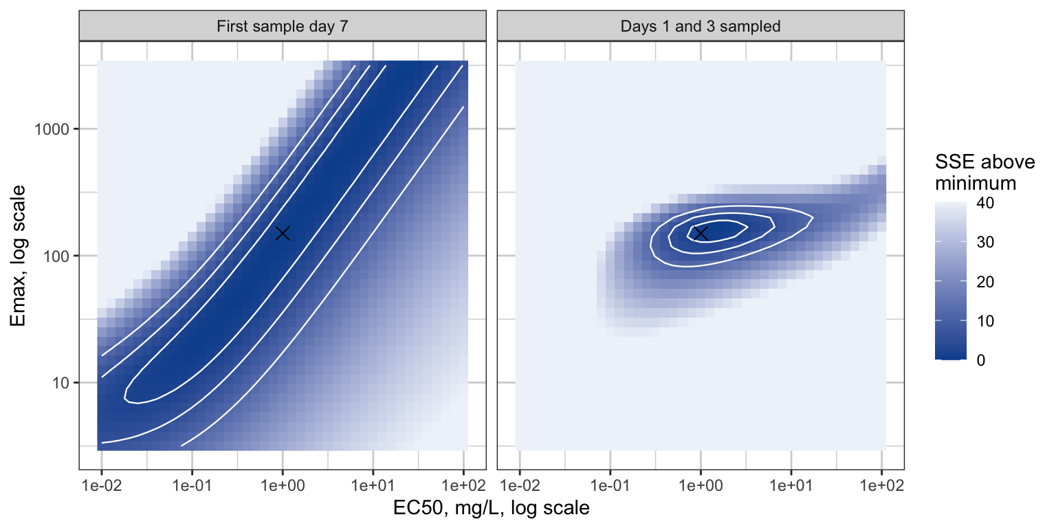
The ridge on the left is the line \(\log E_{\max} - \log EC_{50} =\) constant. Any fitting algorithm started on it stays on it, reports a converged \(E_{\max}\) and \(EC_{50}\) with enormous standard errors or none, and gives the right predictions inside the studied concentration range. That is the situation Dutta et al. described in 1996 for the sigmoid \(E_{\max}\) model with truncated data (references, entry 2): the fit is good, the descriptors inside the data are precise, and \(E_{\max}\) and \(EC_{50}\) are not.
7. What the published models found
| Drug, entry | Patients, doses | Drug effect form | What happened to \(EC_{50}\) | Reference |
|---|---|---|---|---|
| Ofatumumab, 5 | 1,486; 3 to 700 mg across five studies, including 3 and 10 mg arms with partial depletion | Sigmoid \(E_{\max}\) on lysis, within TMDD; \(K_D\) and \(k_{\rm off}\) fixed from preclinical data | Estimated: 0.0057 mg/L, RSE 8.5%; \(E_{\max}\) 159, RSE 3.2% | Yu et al., CNS Drugs 2022, doi |
| Rituximab, paediatric, 6 | 63; full dose; 281 CD19 counts, 52% below the limit | \(E_{\max}\) on degradation, driven by amount | Estimated: \(ED_{50}\) 0.69 mg, RSE 61%, CI 0.18 to 2.26; \(E_{\max}\) 155, CI 153 to 713; authors cite “the highly efficacious doses” | Pharmaceutics 2023;15:2534, doi |
| Inebilizumab, 7 | 213; 0.1 to 10 mg/kg and 30 to 600 mg, a 100-fold range | Log-linear slope on removal | Abandoned: “the estimated EC50 … was less than the assay lower limit of quantitation” | Yan et al., Br J Clin Pharmacol 2022, doi |
| Rituximab, membranous nephropathy, 8 | 41; 375 mg/m² × 4, 1000 mg × 2, 100 mg monthly | TMDD; elimination of the drug-CD20 complex | No \(EC_{50}\); binding constant \(k_{ss}\) at 60% RSE | PMC11002205 |
| Ianalumab, Sjögren’s, 9 | Phase 2 and RA data; 3 and 10 mg/kg single doses in the Phase 2 | Indirect-effect turnover; parameters not public | Not reported; a tissue receptor-occupancy model was added to carry the dose decision | Baltcheva et al., PAGE 2018, abstract |
Three of the five read directly against Sections 4 and 5. Ofatumumab is the case with cohorts in the band: the 3 mg and 10 mg subcutaneous arms gave partial and delayed depletion, subcutaneous absorption slows the fall so that weekly samples see it, and 1,486 patients did the rest. Rituximab at full dose is the ridge, with a 13-fold interval on \(ED_{50}\) and an upper bound on \(E_{\max}\) four times the estimate. Inebilizumab is the ridge recognized and dealt with: the estimator put \(EC_{50}\) below the PK assay, which is where Section 3 says the band is, and the authors fit the slope instead.
Two of the five took the route around the problem: fix the binding constant from in vitro measurements and let the model’s potency come from the literature rather than the data. That is a legitimate answer to “what is \(EC_{50}\)”, and it is not an estimate.
8. The slope parameterization
Schoemaker, van Gerven and Cohen showed in 1998 that when the data do not approach \(E_{\max}\), the parameter \(S_0 = E_{\max}/EC_{50}\), the initial slope of the \(E_{\max}\) curve, is estimable with good precision while its two factors are not, and proposed reporting it (references, entry 1). The inebilizumab model’s \(k = \text{slope} \cdot \log C\) is the same idea in a form that stays finite at high concentration.
For everything downstream of the B-cell count, the slope is enough. The duration of depletion, the time to repopulate to a fraction of baseline, depends on when \(E(C)\) falls to order 1, which is at \(C \approx 1/S_0\), and on \(k_{\rm out}\). Fitting the slope model and the \(E_{\max}\) model to the same sparse data and predicting the duration across the studied dose range:
trep <- function(dose, form = "emax", S = NA, Cref = NA) {
  tt <- seq(0, 500, by = 1)
  B <- sim_B(dose, Emax, EC50, kout, B0, times = tt, form = form, S = S, Cref = Cref)
  i <- which.min(B); j <- which(B[i:length(B)] >= 0.2 * B0)[1]; if (is.na(j)) NA else tt[i + j - 1]
}
Cref <- 0.1
S_match <- Emax / EC50 * Cref     # equal initial slope: S/Cref = Emax/EC50
dd <- 10^seq(-1.5, 2.5, length.out = 17)
tr <- bind_rows(
  data.frame(model = "Emax, EC50 (true)", dose = dd, trep = sapply(dd, trep)),
  data.frame(model = "Log-linear slope",  dose = dd, trep = sapply(dd, trep, form = "slope", S = S_match, Cref = Cref)))
ggplot(tr, aes(dose, trep, colour = model)) +
  annotate("rect", xmin = 3, xmax = 300, ymin = -Inf, ymax = Inf, alpha = 0.08, fill = "grey30") +
  geom_line(linewidth = 0.8) + geom_point(size = 1.8) +
  scale_colour_manual(values = pal3[1:2], name = NULL) +
  scale_x_log10() +
  annotate("text", x = 30, y = 20, label = "studied dose range", size = 3, colour = "grey40") +
  labs(x = "Dose, mg, log scale", y = "Days to repopulate to 20% of baseline") +
  theme(legend.position = "bottom")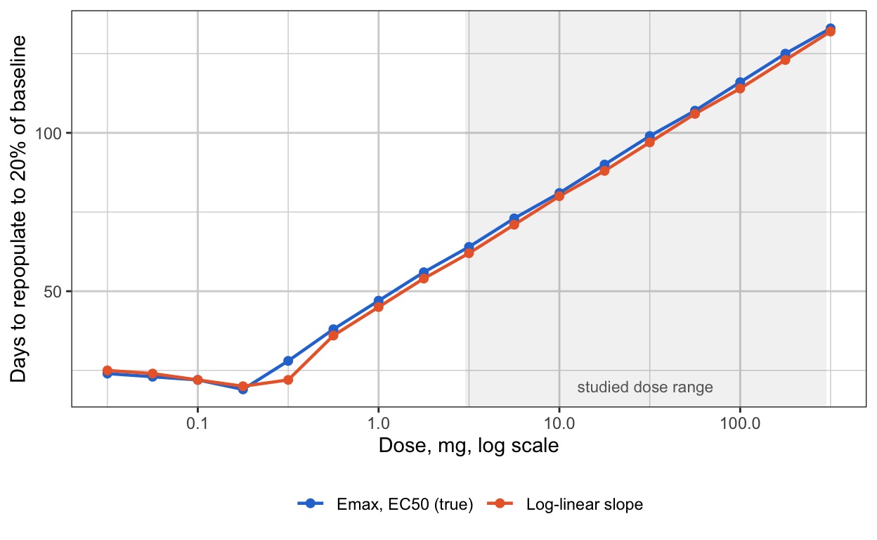
9. What a study needs if it wants EC50
Stated as requirements, in the order they would be dropped from a protocol.
- B-cell samples on days 1 and 3 after the first dose. The speed of the fall is the only observation that separates \(E_{\max}\) from \(EC_{50}\) at a therapeutic dose. With antibody-dependent lysis the fall is hours to days, and a first sample at a week arrives after it.
- B cells monthly until repopulation is complete in most patients. The tail identifies \(k_{\rm out}\), and without \(k_{\rm out}\) the fall identifies nothing.
- A PK assay whose limit is below \(EC_{50}/E_{\max}\), or a willingness to extrapolate the PK tail by a factor of a hundred and say so. Recovery starts at concentrations the assay may never see.
- A cohort at a dose whose nadir is quantifiable and whose concentration sits inside the band of Section 3, if the design can afford one. This is what ofatumumab had. A cohort below the band informs the slope and not the factors; a cohort above it is censored.
- Failing 1 and 4, fit the slope. Report \(S_0\) with its interval, state that \(E_{\max}\) and \(EC_{50}\) are identified as a ratio, and let anyone who needs the factors fix one of them from in vitro binding.
10. What this means for the ITP project
Section 6.2 of the ITP-PK-Platelet specification fits a B-cell layer to a dose escalation of three to six patients per level, first sample at a week, in order to carry the duration of depletion forward to a platelet model. Sections 4 and 5 here say that design identifies the slope and \(k_{\rm out}\) at a usable precision and identifies neither \(E_{\max}\) nor \(EC_{50}\); that Section 8 of the specification is right to parameterize by the slope; and that if the escalation protocol can add days 1 and 3, the \(E_{\max}\) form becomes fittable at about 10% RSE across five cohorts, at the cost of two blood draws.
11. Open questions
- Sigmoidicity. A Hill coefficient above 1 sharpens the band of Section 3 and makes the recovery start more abruptly. Whether it is identifiable alongside the slope at these designs has not been checked.
- Subcutaneous dosing. Absorption over days slows the fall and moves the information of Section 4’s first region into the first week, which is presumably part of why ofatumumab’s model could see it. The simulations here are intravenous.
- Censoring handled properly. Dropping observations below the limit throws away the statement that they are below it. A likelihood with censored terms would recover some information at the floor, and the comparison between designs is not expected to change.
- Between-patient variability. The Fisher information here is for a population with fixed parameters. With 50 to 126% CV on the recovery rate in published models, the precision numbers in Section 5 are optimistic by a factor that a population-design tool would give.