library(nlmixr2)
library(rxode2)
library(ggplot2)
library(dplyr)
theme_set(theme_bw(base_size = 12))Theophylline: data, model, and simulation
Demo page — fitted with nlmixr2 and rxode2
GenAI
demo
The theophylline single-dose dataset plotted, a one-compartment model with first-order absorption fitted with nlmixr2, and the simulation from that fit compared against the observed data.
The data
theo_sd is the theophylline single-dose study: 12 subjects, one oral dose, concentrations followed for 24 hours.
theo <- nlmixr2data::theo_sd
obs  <- theo |> filter(EVID == 0)

obs |>
  ggplot(aes(TIME, DV, group = ID)) +
  geom_line(alpha = 0.4) +
  geom_point(size = 1) +
  labs(x = "Time (h)", y = "Concentration (mg/L)",
       title = "Observed theophylline concentrations, 12 subjects")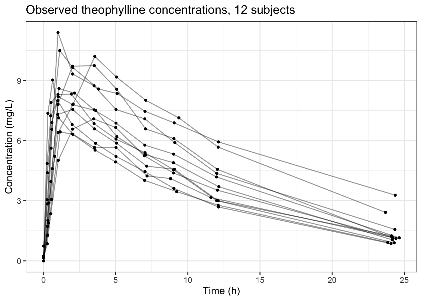
The model
One compartment, first-order absorption, fitted with nlmixr2 using FOCEi.
one.cmt <- function() {
  ini({
    tka <- 0.45   # log ka
    tcl <- 1      # log CL
    tv  <- 3.45   # log V
    eta.ka ~ 0.6
    eta.cl ~ 0.3
    eta.v  ~ 0.1
    add.sd <- 0.7
  })
  model({
    ka <- exp(tka + eta.ka)
    cl <- exp(tcl + eta.cl)
    v  <- exp(tv  + eta.v)
    linCmt() ~ add(add.sd)
  })
}
# The estimation writes progress bars to the console; keep them out of the page.
rxode2::rxSetProgressBar(0)
fit <- suppressMessages(
nlmixr2(one.cmt, theo, est = "focei", control = foceiControl(print = 0))
)knitr::kable(fit$parFixedDf, digits = 3, caption = "Fixed-effect estimates")| Estimate | SE | %RSE | Back-transformed | CI Lower | CI Upper | BSV(CV%) | Shrink(SD)% | |
|---|---|---|---|---|---|---|---|---|
| tka | 0.465 | 0.195 | 41.945 | 1.593 | 1.086 | 2.335 | 70.563 | 1.897 |
| tcl | 1.012 | 0.075 | 7.423 | 2.750 | 2.374 | 3.186 | 26.846 | 4.208 |
| tv | 3.461 | 0.044 | 1.259 | 31.843 | 29.236 | 34.683 | 14.002 | 10.574 |
| add.sd | 0.694 | NA | NA | 0.694 | NA | NA | NA | NA |
Simulation against the observed data
fit |>
  ggplot(aes(TIME, DV)) +
  geom_point(aes(colour = "Observed"), size = 1) +
  geom_line(aes(y = IPRED, colour = "Individual prediction")) +
  geom_line(aes(y = PRED, colour = "Population prediction"), linetype = 2) +
  facet_wrap(~ ID) +
  scale_colour_manual(values = c("Observed" = "black",
                                 "Individual prediction" = "#2c7fb8",
                                 "Population prediction" = "#7fcdbb")) +
  labs(x = "Time (h)", y = "Concentration (mg/L)", colour = NULL,
       title = "Observed data and the fitted model, by subject") +
  theme(legend.position = "bottom")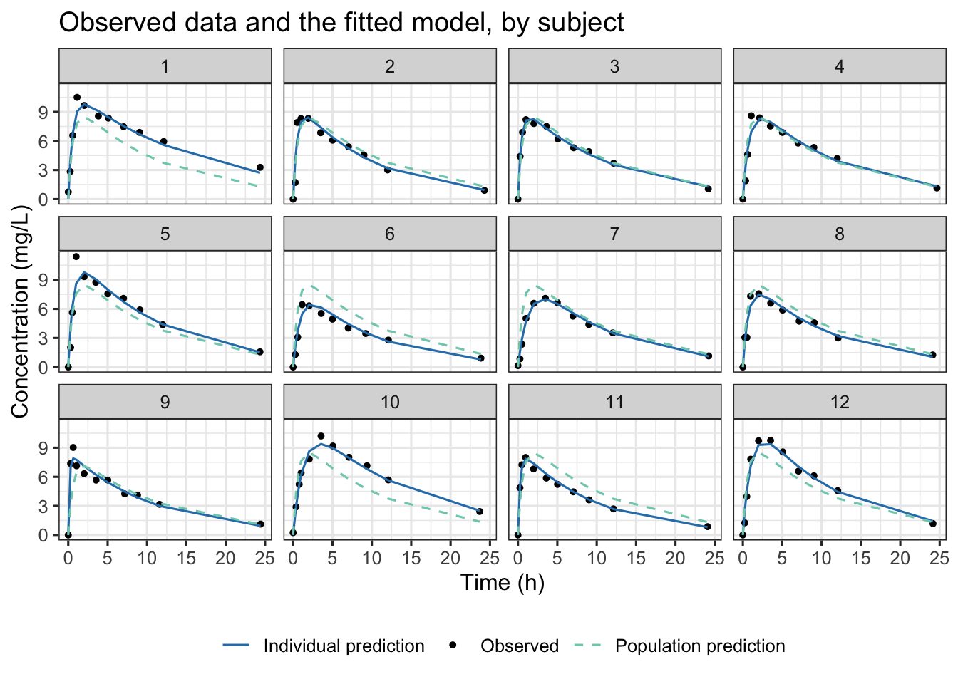
fit |>
  ggplot(aes(IPRED, DV)) +
  geom_abline(slope = 1, intercept = 0, colour = "grey60") +
  geom_point(alpha = 0.7, size = 1) +
  labs(x = "Individual prediction (mg/L)", y = "Observed (mg/L)",
       title = "Observed against individual prediction")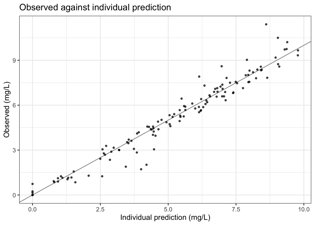
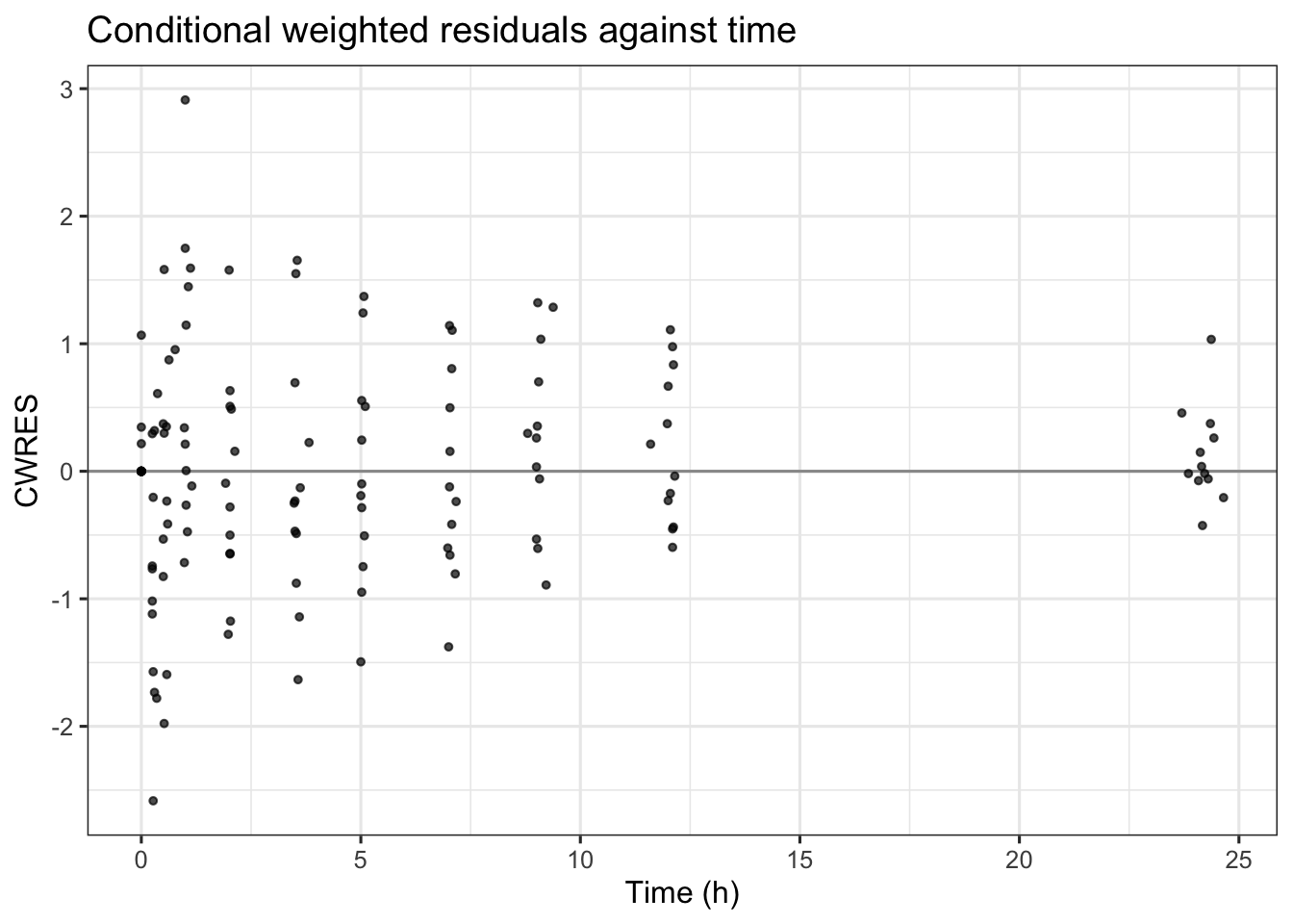
fit |>
  ggplot(aes(TIME, CWRES)) +
  geom_hline(yintercept = 0, colour = "grey60") +
  geom_point(alpha = 0.7, size = 1) +
  labs(x = "Time (h)", y = "CWRES",
       title = "Conditional weighted residuals against time")