library(dplyr)
library(ggplot2)
library(xgxr)

xgx_theme_set()
knitr::opts_chunk$set(fig.height = 4, fig.width = 5)Logistic Regression: Picking a Method
stats::glm, rstanarm, or brms, for a dose-response fit
PMX guide
working document
Comparing three ways to fit a logistic regression of dose against response: the frequentist stats::glm, and two Bayesian options, rstanarm and brms.
Draft, not fully worked through. This compares three ways to fit the same model rather than arguing for one. The glm fit below runs live; the two Bayesian fits do not, because rstanarm and brms are not installed in the environment that builds this site. Their code and Andy’s original conclusions are kept as a record of the comparison, not as a verified result.
1. The Question
Fitting logistic regression for dose against both adverse event rates and overall response rates is a common analysis in dose finding. This page asks whether stats::glm is sufficient, or whether a Bayesian approach through rstanarm or brms is preferable. The same data is fit with three different functions:
stats::glm— frequentist.rstanarm::stan_glm— Bayesian, a package built specifically forglmmodels.brms::brm— Bayesian, using a more flexible modeling package.
Andy’s conclusion from the original comparison: all three gave similar predictions, stats::glm ran fastest and needed no prior specification, so for a quick, exploratory answer stats::glm is the simplest choice. Where strong prior information exists, it should inform the analysis and a Bayesian approach should be used. rstanarm::stan_glm runs faster than brms::brm, because its models are precompiled, and is the more convenient of the two.
2. Caveat: The Limits of Logistic Regression
A binary endpoint carries less information than a continuous one, so a logistic regression fit like the ones below is expected to be of limited value on its own; an analysis with a continuous endpoint will usually be needed to drive dosing decisions. The sizing-studies project works this out in detail. Frank Harrell’s Regression Modeling Strategies gives the quick version: to estimate a baseline rate to within ±10%, at least 96 patients are needed (Section 10.2.2). At the best case, \(p = 0.5\), the variance of the estimate of \(p\) is \(p(1-p)/n\), giving a 95% confidence interval of \(1.96\sqrt{p(1-p)/n} = 0.1\) at \(p = 0.5\) and \(n = 96\).
3. The Data
96 patients from a synthetic Phase 1/2 oncology dataset: assigned dose, baseline covariates, and RECIST-derived response. See the project index for the full column list.
data <- readRDS("../../data/synthetic/dose-response/dose_tumor_resp.rds")

data |>
  group_by(DOSE) |>
  summarise(
    N = n(),
    N_responders = sum(OR == 1, na.rm = TRUE),
    Percent_responders = round(N_responders / N * 100)
  ) |>
knitr::kable(caption = "Response by dose")| DOSE | N | N_responders | Percent_responders |
|---|---|---|---|
| 1 | 2 | 0 | 0 |
| 2 | 1 | 0 | 0 |
| 4 | 1 | 1 | 100 |
| 6 | 3 | 1 | 33 |
| 8 | 14 | 9 | 64 |
| 10 | 9 | 7 | 78 |
| 12 | 10 | 7 | 70 |
| 14 | 5 | 5 | 100 |
| 16 | 51 | 37 | 73 |
4. Frequentist: stats::glm
start_time <- Sys.time()
model <- glm(OR ~ DOSE + ECOG0 + LD0, family = binomial, data = data)
run_time <- Sys.time() - start_time

model |>
  broom::tidy() |>
  arrange(p.value) |>
  select(-statistic) |>
  mutate(
    estimate  = signif(estimate, 2),
    std.error = signif(std.error, 2),
    p.value   = signif(p.value, 2)
  ) |>
  filter(term != "(Intercept)") |>
knitr::kable(caption = "glm coefficient estimates")| term | estimate | std.error | p.value |
|---|---|---|---|
| DOSE | 0.110 | 0.057 | 0.054 |
| LD0 | 0.036 | 0.026 | 0.170 |
| ECOG0 | 0.760 | 0.620 | 0.220 |
ECOG0 is baseline Eastern Cooperative Oncology Group (ECOG) performance status (0 or 1) and LD0 is the baseline sum of target-lesion diameters.
data_sim <- data.frame(
  DOSE = seq(0, 16, by = 0.1), ECOG0 = 1, LD0 = median(data$LD0)
)
p <- predict(model, data_sim, se.fit = TRUE)
f_trans <- function(x) exp(x) / (1 + exp(x))
data_sim$fit   <- f_trans(p$fit)
data_sim$lower <- f_trans(p$fit - 1.96 * p$se.fit)
data_sim$upper <- f_trans(p$fit + 1.96 * p$se.fit)

breaks <- c(0, 7, 11, 13, 16)
g_data <- ggplot(mapping = aes(x = DOSE, y = OR)) +
  geom_jitter(data = data, alpha = 0.5, width = 0, height = 0.1, size = 2) +
  xgx_stat_ci(data = data, distribution = "binomial", breaks = breaks, geom = "point", shape = 0, size = 5) +
  xgx_stat_ci(data = data, distribution = "binomial", breaks = breaks, geom = "errorbar", linewidth = 0.5) +
  scale_x_continuous(breaks = c(0, 4, 8, 12, 16), limits = c(0, 16)) +
  scale_y_continuous(breaks = c(0, 0.5, 1), labels = scales::percent) +
  labs(x = "Dose (mg)", y = "Probability of response")

g_data +
  geom_line(data = data_sim, aes(y = fit), linewidth = 1) +
  geom_ribbon(data = data_sim, aes(ymin = lower, ymax = upper, y = NULL), alpha = 0.25) +
  ggtitle(paste0("Frequentist stats::glm, run time = ", signif(run_time, 2), "s"))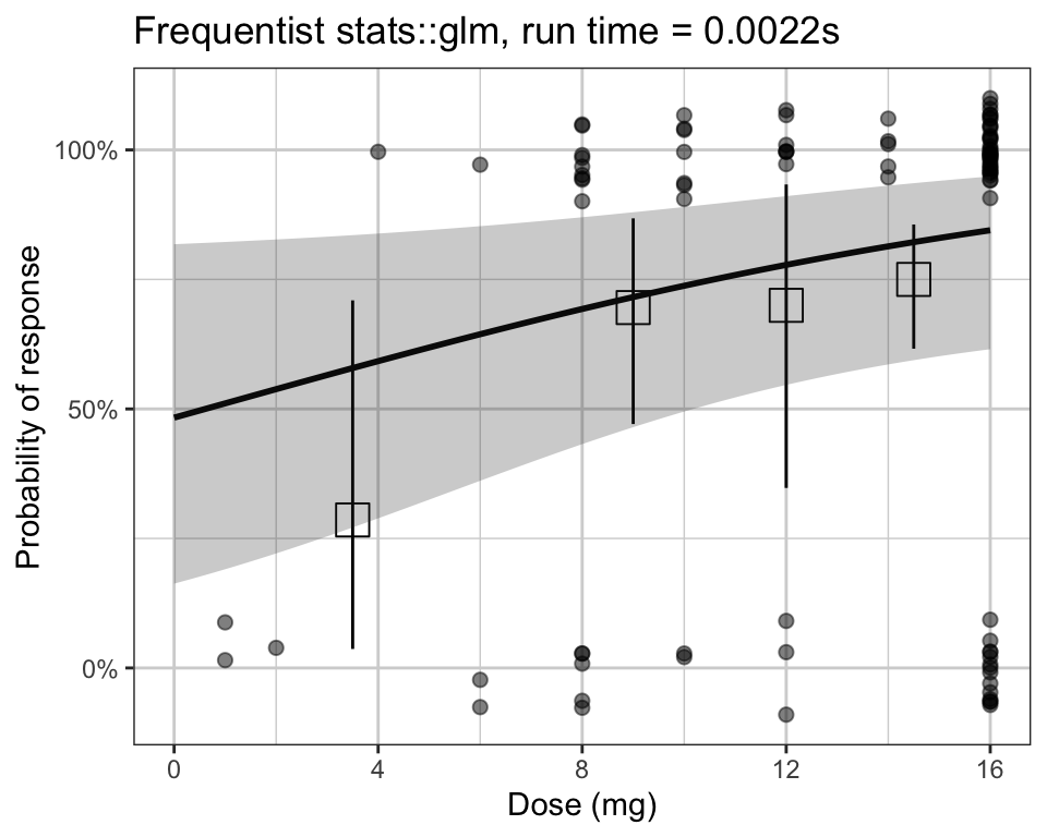
5. Bayesian: rstanarm::stan_glm
rstanarm is not installed in the environment that builds this site, so this chunk does not run. It is kept as the record of what was fit.
library(rstanarm)

fit_rstan <- stan_glm(
  OR ~ DOSE + LD0 + ECOG0,
  data = data,
  family = binomial(link = "logit"),
  prior = normal(c(-2, 0, 0), 3),
  prior_intercept = normal(0.5, 3),
  QR = TRUE,
  seed = 123,
  refresh = 0
)

data_sim <- tibble::tibble(DOSE = seq(0, 16, length.out = 100), ECOG0 = 0, LD0 = median(data$LD0))
p <- predict(fit_rstan, newdata = data_sim, se.fit = TRUE)
data_sim$fit   <- f_trans(p$fit)
data_sim$lower <- f_trans(p$fit - 1.96 * p$se.fit)
data_sim$upper <- f_trans(p$fit + 1.96 * p$se.fit)
6. Bayesian: brms::brm
brms is not installed either. Also kept as a record.
library(brms)

model_blrm <- bf(
  OR ~ beta0 + exp(beta1) * DOSE / 16 + betatum0 * log(LD0) + betaecog * ECOG0,
  beta0 ~ 1, beta1 ~ 1, betatum0 ~ 1, betaecog ~ 1,
  family = bernoulli(), nl = TRUE
)

priors <- c(
  prior(prior = "normal(-2.20, 2)", class = "b", nlpar = "beta0"),
  prior(prior = "normal(-1.02, 1)", class = "b", nlpar = "beta1"),
  prior(prior = "normal(0, 5)",     class = "b", nlpar = "betatum0"),
  prior(prior = "normal(0, 5)",     class = "b", nlpar = "betaecog")
)

blrm_fit <- brm(
  model_blrm, data = data, iter = 7500, warmup = 2500,
  seed = 9999, chains = 4, prior = priors, cores = 4
)
7. Acknowledgements
Thanks to Juan Gonzalez-Maffe for the original brms code, and to Sebastian Weber, Lukas Widner and Andrew Bean for help understanding these options.