| True population response rate | Chance of at least 9/10 responders |
|---|---|
| 50.0% | 1.1% |
| 70.0% | 14.9% |
| 80.0% | 37.6% |
| 85.0% | 54.4% |
| 90.0% | 73.6% |
| 95.0% | 91.4% |
A Model-Based Comparison for Three Cohorts of Ten
Response rates, dose selection and evidence that the population meets the target
Dose-response methods
simulation
Reproducible binomial calculations and simulations comparing observed responder counts with continuous biomarker models, including misspecified dose-response and variance assumptions.
Continuous-data modeling can improve this decision, but the benefit depends on the assumptions used to share information. The calculations below keep the response definition fixed: at least an 80% biomarker decline at a prespecified assessment, with a target population response rate of 90%.
These are synthetic, single-assessment examples. They do not quantify the additional benefit of pharmacokinetics (PK) or longitudinal pharmacodynamics (PD). The specification defines those comparisons; the literature review explains their published basis.
1. What Nine Responders Out of Ten Establishes
If patients independently respond with probability \(p\), the probability that the observed cohort passes is
\[ P(K\ge9\mid p)=10p^9(1-p)+p^{10},\qquad K\sim\mathrm{Binomial}(10,p). \]
A cohort with a true response rate of 80% passes the rule 37.6% of the time. At exactly the 90% population target, the observed cohort fails 26.4% of the time. These are properties of the rule, before introducing any model.
When three independent cohorts all have a true response rate of 80%, at least one passes with probability \(1-\{1-P(K\ge9\mid p=0.8)\}^3\) = 75.7%. Selecting any passing dose therefore requires evaluating the whole selection procedure, including the opportunity to pass at several doses.
| Observed responders | One-sided 95% exact lower bound on p | Pr(p >= 90% | data), uniform Beta(1,1) prior |
|---|---|---|
| 9/10 | 60.6% | 30.3% |
| 10/10 | 74.1% | 68.6% |
The confidence bound and the Bayesian probability answer different questions; the latter depends on the stated prior. Neither analysis of 9/10 establishes the population target with high certainty. Even 10/10 cannot reject \(H_0:p\le0.9\) in a conventional, nonrandomized one-sided 5% exact binomial test: its smallest attainable p-value is \(0.9^{10}\) = 34.9%. With all successes, at least 29 patients at one dose are needed for the one-sided 95% exact lower bound to exceed 90%. This is an all-success bound, not a powered sample size recommendation.
2. Estimating the Same Response Rate From Continuous Data
Define \(Y=\log\{B(t^*)/B(0)\}\), where \(B\) is a positive biomarker and \(t^*\) is the assessment time. An 80% decline corresponds to \(Y\le c=\log(0.2)\). Under the illustrative model \(Y\mid d\sim N\{\mu(d),\sigma(d)^2\}\),
\[ p(d)=\Phi\!\left(\frac{c-\mu(d)}{\sigma(d)}\right). \]
The fitted mean and the spread both determine the responder fraction. Estimating only the mean decline, or counting responders among fitted individual means after shrinkage, does not calculate this population quantity. The normal model here describes observed log ratios, so its standard deviation (SD) includes all variation in that observed endpoint.
For a single dose, the large-sample variance of the plug-in estimate is approximately
\[ \operatorname{Var}(\widehat p_{\rm continuous}) \approx\frac{\phi(z)^2}{n}\left(1+\frac{z^2}{2}\right), \quad z=\Phi^{-1}(p). \]
The \(z^2/2\) term accounts for estimating the standard deviation. It follows by applying the delta method to the sample mean and standard deviation of normal data. The binary estimator has variance \(p(1-p)/n\). The ratio of these variances is an approximate ratio of required sample sizes for equally precise estimation of \(p\).
| True response rate | Binary / continuous variance, SD estimated | Binary / continuous variance, SD known |
|---|---|---|
| 50.0% | 1.57 | 1.57 |
| 80.0% | 1.51 | 2.04 |
| 90.0% | 1.60 | 2.92 |
| 95.0% | 1.90 | 4.47 |
At \(p=0.9\), the estimated-SD calculation gives an efficiency factor of 1.6, equivalent asymptotically to a 37.7% sample size reduction for this estimation problem. Treating the SD as known would exaggerate the gain when it must be learned from these patients. These calculations are neither a finite-sample power result nor an additional benefit from PK. The distributional-estimation idea goes back at least to Suissa (1991); the calculation above is independently implemented for this example.
3. Comparing Dose Decisions
Each simulated study has ten independent patients at each of three relative doses, 1, 2 and 4. There is one observed log biomarker ratio per patient, complete follow-up, and no assay censoring. All methods receive the same patients. The decision is to select the lowest tested dose whose estimated response probability reaches 90%, or select no dose if none qualifies.
| Method | Information and assumptions |
|---|---|
| M0 Counts | Separate responder proportions. A dose passes at 9/10 or 10/10. |
| M1 Binary monotone | Isotonic binomial estimates: pool neighboring arms only when their observed response rates decrease with dose. |
| M2 Continuous per arm | Separate normal mean and SD for each dose’s log ratio. |
| M3 Shared SD | Separate means, with a common residual SD estimated from all three arms. |
| M4 Dose curve | A straight line for mean log ratio against log dose, with a common residual SD. |
M2 isolates the gain from retaining response magnitudes. M3 shares variance information. M4 also shares information about the means. With equal cohort sizes, isotonic least squares on the observed proportions gives the order-restricted binomial maximum likelihood estimates used in M1. M4’s slope is unconstrained; a reversal can be fitted. Its log-dose shape only applies over the tested range and is not a mechanistic dose model.
| Scenario | Dose 1: p (SD) | Dose 2: p (SD) | Dose 4: p (SD) |
|---|---|---|---|
| Smooth: middle qualifies | 76.0% (SD 0.45) | 92.0% (SD 0.45) | 98.2% (SD 0.45) |
| Smooth: high qualifies | 69.0% (SD 0.45) | 84.0% (SD 0.45) | 93.2% (SD 0.45) |
| Plateau: none qualifies | 85.0% (SD 0.45) | 85.0% (SD 0.45) | 85.0% (SD 0.45) |
| Late rise: high qualifies | 45.0% (SD 0.45) | 65.0% (SD 0.45) | 97.0% (SD 0.45) |
| Unequal SD: none qualifies | 75.0% (SD 0.2) | 84.0% (SD 0.4) | 89.0% (SD 0.9) |
The first two scenarios satisfy M4’s shape and common-SD assumptions. The plateau also satisfies the linear model, with zero slope. The late-rise scenario violates the linear mean shape. The last scenario violates both M4’s mean shape and the shared-SD assumption; all doses are inadequate. M2 remains correctly specified in every scenario because the log ratios within each arm are normal.
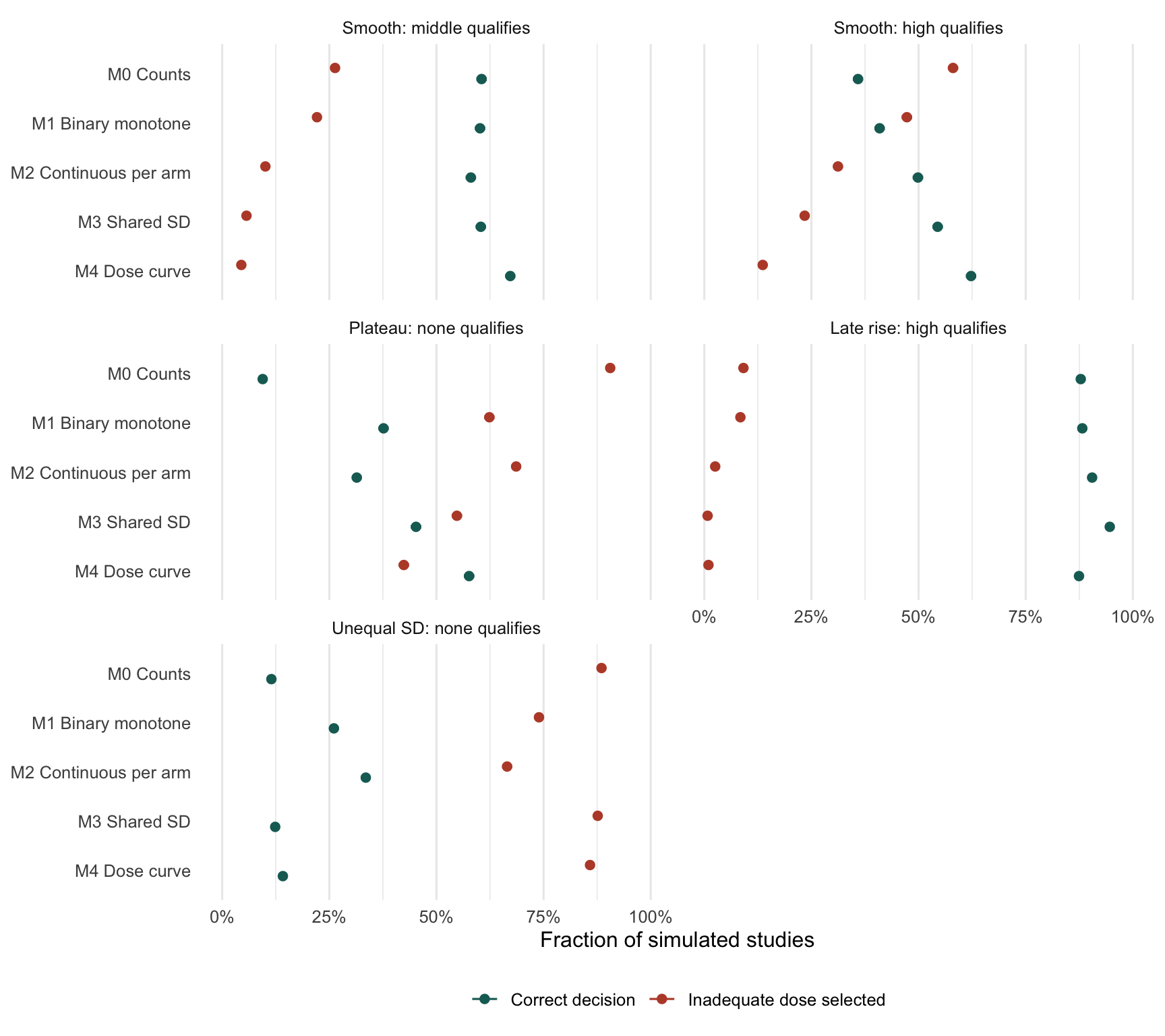
When only the high dose qualifies under a smooth curve, correct selection rises from 35.9% with counts to 62.3% with the dose curve. In the late-rise scenario, the shared-SD model with separate means does better than imposing the linear mean shape. In the unequal-SD scenario, variance pooling makes the decision worse.
The point-estimate rules do not control a 5% false-positive rate. Their different false-positive rates also mean that the difference in correct selection cannot be called a gain in statistical power at equal type I error. Precision, decision accuracy and evidence against a null hypothesis are separate comparisons.
NoteAll Point-Estimate Decisions
| Scenario | Method | Correct decision | Inadequate dose | Higher adequate dose | No dose |
|---|---|---|---|---|---|
| Smooth: middle qualifies | M0 Counts | 60.5% | 26.3% | 13.0% | 0.1% |
| Smooth: middle qualifies | M1 Binary monotone | 60.2% | 22.1% | 17.1% | 0.6% |
| Smooth: middle qualifies | M2 Continuous per arm | 58.0% | 10.1% | 31.1% | 0.8% |
| Smooth: middle qualifies | M3 Shared SD | 60.4% | 5.7% | 33.4% | 0.6% |
| Smooth: middle qualifies | M4 Dose curve | 67.2% | 4.5% | 27.7% | 0.6% |
| Smooth: high qualifies | M0 Counts | 35.9% | 58.0% | 0.0% | 6.1% |
| Smooth: high qualifies | M1 Binary monotone | 40.9% | 47.3% | 0.0% | 11.8% |
| Smooth: high qualifies | M2 Continuous per arm | 49.9% | 31.2% | 0.0% | 19.0% |
| Smooth: high qualifies | M3 Shared SD | 54.4% | 23.4% | 0.0% | 22.1% |
| Smooth: high qualifies | M4 Dose curve | 62.3% | 13.6% | 0.0% | 24.1% |
| Plateau: none qualifies | M0 Counts | 9.4% | 90.5% | 0.0% | 9.4% |
| Plateau: none qualifies | M1 Binary monotone | 37.6% | 62.4% | 0.0% | 37.6% |
| Plateau: none qualifies | M2 Continuous per arm | 31.4% | 68.6% | 0.0% | 31.4% |
| Plateau: none qualifies | M3 Shared SD | 45.2% | 54.8% | 0.0% | 45.2% |
| Plateau: none qualifies | M4 Dose curve | 57.6% | 42.4% | 0.0% | 57.6% |
| Late rise: high qualifies | M0 Counts | 87.8% | 9.1% | 0.0% | 3.0% |
| Late rise: high qualifies | M1 Binary monotone | 88.2% | 8.4% | 0.0% | 3.4% |
| Late rise: high qualifies | M2 Continuous per arm | 90.5% | 2.5% | 0.0% | 7.0% |
| Late rise: high qualifies | M3 Shared SD | 94.6% | 0.8% | 0.0% | 4.6% |
| Late rise: high qualifies | M4 Dose curve | 87.4% | 1.0% | 0.0% | 11.6% |
| Unequal SD: none qualifies | M0 Counts | 11.5% | 88.5% | 0.0% | 11.5% |
| Unequal SD: none qualifies | M1 Binary monotone | 26.1% | 73.9% | 0.0% | 26.1% |
| Unequal SD: none qualifies | M2 Continuous per arm | 33.5% | 66.5% | 0.0% | 33.5% |
| Unequal SD: none qualifies | M3 Shared SD | 12.4% | 87.6% | 0.0% | 12.4% |
| Unequal SD: none qualifies | M4 Dose curve | 14.2% | 85.8% | 0.0% | 14.2% |
When all doses are inadequate, a correct decision and a no-dose decision are the same event. Those two columns therefore overlap in those scenarios. In scenarios with an adequate dose, the four columns partition the decisions.
4. Requiring Evidence That a Dose Exceeds the Target
A second comparison asks for evidence against \(H_0:p(d)\le0.9\). Every method receives a one-sided error allowance of \(0.05/3\) per tested dose. The Bonferroni bound limits the chance of declaring any truly inadequate dose to at most 5%, provided each model’s test is valid. The lowest dose that rejects its null is selected.
For normal data with fitted mean \(\widehat\mu_d\), residual SD \(s\), residual degrees of freedom \(\nu\), and mean-variance factor \(h_d=\operatorname{Var}(\widehat\mu_d)/\sigma^2\),
\[ T_d=\frac{c-\widehat\mu_d}{s\sqrt{h_d}} \sim t_\nu\!\left(\frac{z_d}{\sqrt{h_d}}\right), \qquad z_d=\Phi^{-1}\{p(d)\}. \]
The noncentral-\(t\) distribution gives an exact upper critical value at \(z_d=\Phi^{-1}(0.9)\). This accounts for uncertainty in the fitted mean and SD. M2 uses \(h_d=1/10\), \(\nu=9\); M3 uses \(h_d=1/10\), \(\nu=27\); M4 uses the regression prediction variance and \(\nu=28\). The binary comparator uses an exact binomial test. M1 is omitted from this comparison because an order-restricted testing procedure has not been implemented.
| Scenario | Method | Correct decision | Inadequate dose | Higher adequate dose | No dose |
|---|---|---|---|---|---|
| Smooth: middle qualifies | M0 Counts | 0.0% | 0.0% | 0.0% | 100.0% |
| Smooth: middle qualifies | M2 Continuous per arm | 2.7% | 0.1% | 19.3% | 77.9% |
| Smooth: middle qualifies | M3 Shared SD | 3.4% | 0.0% | 39.9% | 56.7% |
| Smooth: middle qualifies | M4 Dose curve | 4.6% | 0.0% | 43.5% | 51.9% |
| Smooth: high qualifies | M0 Counts | 0.0% | 0.0% | 0.0% | 100.0% |
| Smooth: high qualifies | M2 Continuous per arm | 3.6% | 0.5% | 0.0% | 95.9% |
| Smooth: high qualifies | M3 Shared SD | 5.3% | 0.2% | 0.0% | 94.5% |
| Smooth: high qualifies | M4 Dose curve | 5.6% | 0.1% | 0.0% | 94.3% |
| Plateau: none qualifies | M0 Counts | 100.0% | 0.0% | 0.0% | 100.0% |
| Plateau: none qualifies | M2 Continuous per arm | 98.4% | 1.6% | 0.0% | 98.4% |
| Plateau: none qualifies | M3 Shared SD | 99.0% | 1.0% | 0.0% | 99.0% |
| Plateau: none qualifies | M4 Dose curve | 99.5% | 0.5% | 0.0% | 99.5% |
| Late rise: high qualifies | M0 Counts | 0.0% | 0.0% | 0.0% | 100.0% |
| Late rise: high qualifies | M2 Continuous per arm | 11.3% | 0.0% | 0.0% | 88.6% |
| Late rise: high qualifies | M3 Shared SD | 23.5% | 0.0% | 0.0% | 76.5% |
| Late rise: high qualifies | M4 Dose curve | 11.8% | 0.0% | 0.0% | 88.2% |
| Unequal SD: none qualifies | M0 Counts | 100.0% | 0.0% | 0.0% | 100.0% |
| Unequal SD: none qualifies | M2 Continuous per arm | 98.2% | 1.8% | 0.0% | 98.2% |
| Unequal SD: none qualifies | M3 Shared SD | 66.4% | 33.6% | 0.0% | 66.4% |
| Unequal SD: none qualifies | M4 Dose curve | 74.8% | 25.2% | 0.0% | 74.8% |
The binary test cannot pass with ten patients per dose, as Section 1 showed. The normal-data tests can pass because they also observe how far the responses lie beyond the threshold. Their power is still limited close to the population target. A more distant, clearly adequate high dose is easier to certify than the lowest adequate dose.
The apparent certainty can fail under misspecification. In the unequal-SD scenario, M3 selects an inadequate dose in 33.6% of studies despite its nominal 5% familywise allowance. M2’s corresponding rate is 1.8%. This is why an integrated model needs a calibrated decision rule and plausible misspecification scenarios before a claim about sample savings.
5. Reproduction and Next Comparison
The R source contains the settings, generators, estimators, decision rules and numerical checks. This page reruns the calculations at render time. The simulation uses 10,000 replicates per scenario and seed 20260922. At that simulation size, the largest possible Monte Carlo standard error for a reported proportion is 0.50 percentage points; uncertainty about the scenario parameters is not included.
The run also returns dose-specific bias and root mean squared error in benchmark$estimates. The analytical checks verify the binomial tail, confidence-bound calculation, no-dose selection and the noncentral-\(t\) test’s boundary rejection rate by numerical integration.
The next comparison adds repeated biomarker measurements, followed by PK, using the same target and decision rules. Those additions must improve on M2–M4 to establish an incremental benefit from integrated pharmacometric modeling.