library(ggplot2)
library(dplyr)
library(xgxr)

set.seed(12345)
xgx_theme_set()
knitr::opts_chunk$set(fig.height = 4, fig.width = 5)Sizing Studies for Dose-Response Characterization
How many patients an expansion cohort needs to see a dose-response or biomarker-response relationship
PMX guide
Four approaches to sizing a Phase 1/2 oncology cohort against a dose-response or biomarker-response endpoint: Frank Harrell’s p < m/15 rule, Richard Riley’s four-question framework, worked binary and continuous examples, and why a continuous endpoint is usually the practical choice.
This estimates how many patients a cohort needs to characterize a dose-response or biomarker-response relationship with useful precision. It does not size a study to reject a null hypothesis that two doses are the same — Section 1 explains why that is usually the wrong question — and it does not cover Phase 3 confirmatory sizing.
1. Why the Usual Power Calculation Is the Wrong Question
The main purpose of a Phase 1 study is to assess the safety of a drug. It is important to start from a first-in-human dose expected to be safe, and the goal is often to identify a maximum tolerated dose (MTD), though for many biologics — pembrolizumab and nivolumab, for example — the drug is safe enough across the tested range that an MTD cannot be identified.
After the MTD, or some other maximum allowable dose set by a constraint such as manufacturability or cost of goods, the next step is choosing the dose or doses to test in expansion cohorts, and how many patients each cohort needs. That data then informs the dose or doses carried into later studies. The FDA’s 2023 draft guidance on dose optimization in oncology trials states that “the trial should be sized to allow for sufficient assessment of activity, safety, and tolerability for each dosage. The trial does not need to be powered to demonstrate statistical superiority of a dosage or statistical non-inferiority among the dosages” (FDA 2023), without saying what “sufficient assessment” means.
Three considerations bear on choosing the number and size of the expansion cohorts:
- The goal is generally not to reject the null hypothesis that two doses are identical. At reasonable dose choices, most drugs show some difference in safety and efficacy between two doses; the question is how large that difference is and whether it is detectable. Pembrolizumab and nivolumab are the notable exception, where both tested doses saturated PD-1.
- The FDA restricts expansion cohorts to at most 40 patients in solid tumor indications, or 20 in a hematological malignancy rare enough to support initiating efficacy trials on a smaller efficacy database (FDA 2022).
- The FDA recommends randomization for comparing activity across different dosing regimens within a cohort (FDA 2022).
On efficacy assessment specifically, the FDA guidance states that “the analysis plan for each expansion cohort should contain adequate information justifying the planned sample size based on the cohort objectives. For those cohorts evaluating antitumor activity, the plans should specify the magnitude of antitumor activity that would warrant further evaluation of the drug, for example by specifying the precision and power considerations for detection of clinically meaningful antitumor activity. In general, in a nonrandomized cohort, assessment of antitumor activity is determined using a Simon two-stage design or other designs (e.g., Bayesian statistical design) to limit exposure of additional subjects to a potentially ineffective drug” (FDA 2022).
2. Estimating Dose-Response With Sufficient Precision
Methodology
The FDA guidance (FDA 2022) caps expansion cohorts at 20 to 40 patients. Could a leaner study still learn enough to tell which of two doses is better to carry forward, especially with a validated biomarker that predicts long-term response well? Four approaches to sizing such a study follow.
Frank Harrell’s m/15 Heuristic
In Regression Modeling Strategies, Section 4.4 (Harrell 2015), Frank Harrell recommends that the number of model parameters \(p\) stay below one fifteenth of the effective sample size \(m\): \(p < m/15\), where \(m\) is:
- For a continuous endpoint, the total number of patients.
- For a binary endpoint, the smaller of the number of responses and the number of non-responses.
- For a time-to-event endpoint, the number of failures.
- For an ordinal endpoint, a calculation slightly more complex than the above, not covered here.
Richard Riley’s Four Questions
A more rigorous set of criteria for the minimum sample size of a prediction model is set out in Riley et al. 2020, with the full derivations in two companion papers, for continuous endpoints (Riley et al. 2019a) and for binary and time-to-event endpoints (Riley et al. 2019b). When a study is designed to use multiple factors to predict response — dose and biomarker expression, say — four questions should set the sample size:
- What sample size gives a precise estimate of the overall outcome risk or mean outcome value?
- What sample size gives predicted values with a small mean error across all individuals?
- What sample size keeps the required shrinkage of predictor effects small, reducing the risk of overfitting?
- What sample size keeps the optimism in apparent model fit small — that is, keeps the calculated \(R^2\) close to the true \(R^2\), which also reduces overfitting?
One more question in this context: is 40 patients per arm enough to characterize the dose-response relationship? For a binary or categorical endpoint, 40 may not be, though it is still a reasonable starting point.
Trial Simulation
Section 10.2.3 of Harrell 2015 gives a trial simulation calculation for a binary endpoint depending on one variable: pick the sample size so the expected maximum error in the estimated probability of response, given the variable, stays under some value. As with the approaches above, the goal is not to estimate power and accept or reject a null hypothesis — it is to estimate the function relating the independent variables to the endpoint, to within a stated error. Since the goal of a Phase 1-2 study is to learn the dose-exposure-biomarker-response relationship for safety and efficacy, minimizing the error in the model prediction is a reasonable criterion for the required study size, though this document does not explore the approach further.
3. Binary Response Example: Overall Response Rate
Harrell’s Rule of Thumb
For a dose-response model, at least two parameters are needed (a linear model, with slope and intercept), and ideally three (an Emax model, with \(E_0\), \(E_\text{max}\), and \(ED_{50}\)). Applying Harrell’s \(p < m/15\) rule, where the probability of response \(p_\text{resp} \le 0.5\):
\[ \begin{align*} p & < \frac{m}{15} = \frac{p_\text{resp} \cdot n}{15} \\ n & > \frac{15\,p}{p_\text{resp}} \end{align*} \]
data.frame(
  model     = c("Linear", "Linear", "Emax", "Emax"),
  p         = c(2, 2, 3, 3),
  prob_resp = c(0.2, 0.5, 0.2, 0.5)
) |>
  mutate(n_patients = round(15 * p / prob_resp)) |>
knitr::kable(caption = "Minimum patients by model and response rate")| model | p | prob_resp | n_patients |
|---|---|---|---|
| Linear | 2 | 0.2 | 150 |
| Linear | 2 | 0.5 | 60 |
| Emax | 3 | 0.2 | 225 |
| Emax | 3 | 0.5 | 90 |
The minimum is 60 patients, for a linear dose-response model and a 50% response rate. A study cannot generally count on a linear model being sufficient, and should plan for the possibility that an Emax model is required — in which case 150 to 225 patients are needed, more than most first-in-human studies enroll.
Riley’s Approach
Using the more rigorous approach for a binary outcome (Riley et al. 2019b), the 95% confidence interval for an event rate \(p\) is
\[ p \pm \delta, \quad \delta = 1.96 \sqrt{\frac{p(1-p)}{n}} \]
Solving for \(n\):
\[ n = \left( \frac{1.96}{\delta} \right)^2 p(1-p) \]
data.frame(delta = c(0.05, 0.05, 0.1, 0.1), p = c(0.2, 0.5, 0.2, 0.5)) |>
  mutate(n = round((1.96 / delta)^2 * p * (1 - p))) |>
knitr::kable(caption = "Patients needed for a given confidence-interval width")| delta | p | n |
|---|---|---|
| 0.05 | 0.2 | 246 |
| 0.05 | 0.5 | 384 |
| 0.10 | 0.2 | 61 |
| 0.10 | 0.5 | 96 |
At \(\delta = 0.05\), over 200 patients are needed, impractical for a first-in-human oncology study. At \(\delta = 0.1\), 60 to 100 patients is more reasonable — but that is only the calculation for the overall event rate in one arm. If the response rate between two dose groups is expected to differ by only 10 to 20 percentage points, \(\delta = 0.1\) is too wide to detect that difference.
Why a Binary Endpoint Is Not Enough
Both the Harrell rule of thumb and the Riley approach put the sample size needed to estimate a binary dose-response relationship in the hundreds of patients. This is why, when using a first-in-human oncology trial to select doses for further study, a continuous endpoint is needed: it gives greater precision for detecting a difference between two doses with the same number of patients.
4. Continuous Response Example: Percent Change in Tumor Size
Example Data
Sizing a study for a continuous endpoint needs some knowledge of the endpoint’s properties. Below, an Emax model is fit to percent change in tumor size at the first on-treatment assessment, in 61 patients from a synthetic Phase 1/2 oncology dataset (see the project index for what it holds).
data <- readRDS("../../data/synthetic/dose-response/emax_tumor_size.rds") |>
  rename(Dose = Average_Dose)

mod <- stats::nls(
  Tumor_Pct_Change ~ E0 + Emax * Dose / (ED50 + Dose),
  data  = data,
  start = list(E0 = 40, Emax = -120, ED50 = 200)
)

data <- data |>
  mutate(Tumor_Pct_Change_Pred = predict(mod))

sd0      <- sd(data$Tumor_Pct_Change)
sd_tumor <- sd(data$Tumor_Pct_Change - data$Tumor_Pct_Change_Pred)
r2       <- 1 - sd_tumor^2 / sd0^2

ggplot(data, aes(x = Dose, y = Tumor_Pct_Change)) +
  geom_point() +
  xgx_stat_smooth(
    method = "nlsLM", formula = y ~ E0 + Emax * x / (ED50 + x),
    method.args = list(start = list(Emax = -120, ED50 = 200, E0 = 40)),
    se = TRUE
  ) +
  labs(
    x = "Average daily dose before first assessment",
    y = "Percent change in tumor size\nat first assessment",
    title = paste0(
      "N = ", nrow(data), ", SD = ", signif(sd_tumor, 3),
      "%, R² = ", signif(r2, 3)
    )
  ) +
  scale_y_continuous(limits = c(-100, 60), breaks = seq(-100, 60, by = 20))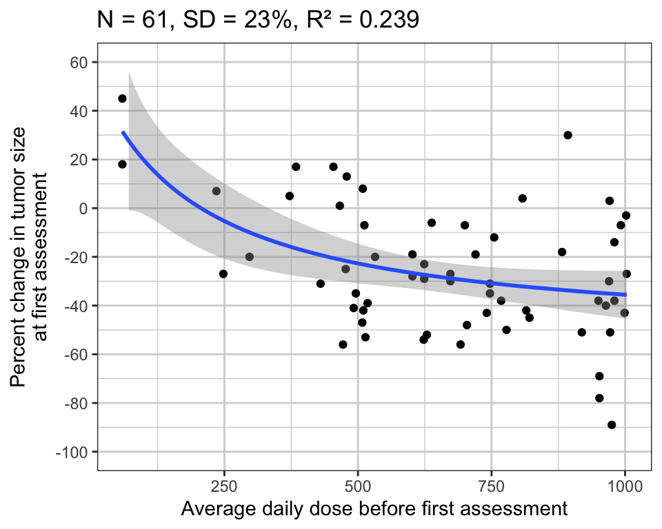
Harrell’s Rule of Thumb
For a continuous endpoint, Harrell’s rule needs only 15 patients per parameter — a much smaller requirement than for a binary endpoint — with 30 to 45 patients needed for the linear and Emax models.
data.frame(model = c("Linear", "Emax"), p = c(2, 3)) |>
  mutate(n_patients = round(15 * p)) |>
knitr::kable(caption = "Minimum patients by model, continuous endpoint")| model | p | n_patients |
|---|---|---|
| Linear | 2 | 30 |
| Emax | 3 | 45 |
Riley’s Approach, Four Steps
The calculations below directly implement Riley et al. 2019a. The reference explains each calculation in full; the summary here does not.
Step 1: Calculating Shrinkage
For a 3-parameter model, an apparent \(R^2\) within 90% of the adjusted \(R^2\) needs about 50 patients. A more complex model relating both dose and a biomarker to response, with 5 to 6 parameters, needs around 100.
shrinkage <- expand.grid(
  n     = 1:100,
  R2app = c(0.1, 0.25, 0.5),
  p     = c(3, 4, 5, 6)
) |>
  mutate(
    S_C = 1 + (p - 2) / (n * log(1 - R2app)),        # Equation 6 of Riley et al. 2019a
    R2app_str = paste0("R2app = ", R2app)
  )

ggplot(shrinkage, aes(x = n, y = S_C, color = factor(p))) +
  geom_line() +
  ylim(0, 1) +
  geom_hline(yintercept = 0.9, linetype = "dashed") +
  labs(x = "Number of patients", y = "Copas shrinkage factor", color = "N param.") +
  facet_wrap(~R2app_str)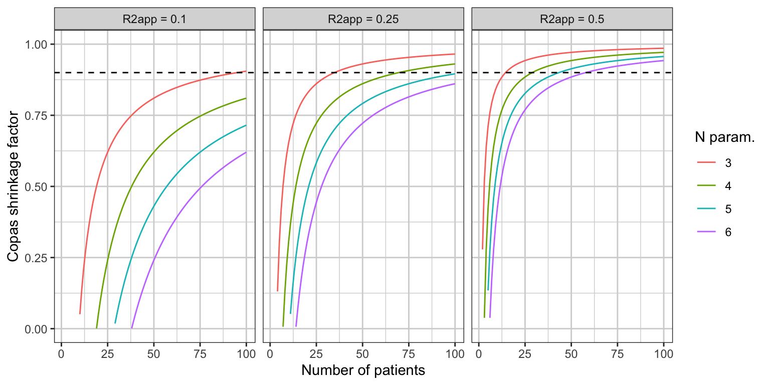
Step 2: N for Apparent R² Close to Adjusted R²
The number of patients needed here also depends on \(R^2\) and the parameter count. For a 3-parameter Emax model with \(R^2 = 0.25\), only 46 patients are needed; a 5- to 6-parameter model that also describes the biomarker-response relationship needs 70 to 90.
expand.grid(R2 = c(0.1, 0.25, 0.5), p = c(3, 4, 5, 6), delta = 0.05) |>
  mutate(n = round(1 + p * (1 - R2) / delta)) |>
knitr::kable(caption = "Patients needed for apparent R² within delta of adjusted R²")| R2 | p | delta | n |
|---|---|---|---|
| 0.10 | 3 | 0.05 | 55 |
| 0.25 | 3 | 0.05 | 46 |
| 0.50 | 3 | 0.05 | 31 |
| 0.10 | 4 | 0.05 | 73 |
| 0.25 | 4 | 0.05 | 61 |
| 0.50 | 4 | 0.05 | 41 |
| 0.10 | 5 | 0.05 | 91 |
| 0.25 | 5 | 0.05 | 76 |
| 0.50 | 5 | 0.05 | 51 |
| 0.10 | 6 | 0.05 | 109 |
| 0.25 | 6 | 0.05 | 91 |
| 0.50 | 6 | 0.05 | 61 |
Step 3: A Reasonable Estimate for the Variance
The number of patients needed to estimate the variance to within 20% or 10% comes directly from the \(\chi^2\) distribution:
- \(70 + p\) for the variance within 20% of the true value, at 95% confidence.
- \(234 + p\) for the variance within 10% of the true value, at 95% confidence.
Step 4: A Reasonable Estimate for the Mean
The inverse \(t\) distribution gives the 5th to 95th percentile confidence interval directly:
\[ t\!\left(1 - \frac{0.05}{2},\; n - p - 1\right) \cdot \frac{\sigma}{\sqrt{n}} \]
expand.grid(n = c(40, 60, 100, 200), p = c(3, 4, 5, 6)) |>
  mutate(ci95 = signif(qt(1 - 0.05 / 2, n - p - 1) * sd_tumor / sqrt(n), 4)) |>
knitr::kable(caption = "95% CI half-width on the mean, by N and parameter count")| n | p | ci95 |
|---|---|---|
| 40 | 3 | 7.364 |
| 60 | 3 | 5.939 |
| 100 | 3 | 4.558 |
| 200 | 3 | 3.202 |
| 40 | 4 | 7.371 |
| 60 | 4 | 5.941 |
| 100 | 4 | 4.559 |
| 200 | 4 | 3.203 |
| 40 | 5 | 7.379 |
| 60 | 5 | 5.944 |
| 100 | 5 | 4.560 |
| 200 | 5 | 3.203 |
| 40 | 6 | 7.387 |
| 60 | 6 | 5.946 |
| 100 | 6 | 4.560 |
| 200 | 6 | 3.203 |
At \(\sigma \approx 20\%\) in this example, this step was not the limiting constraint.
Power of a Continuous Endpoint
Fitting only a 3-parameter Emax model, 40 to 50 patients can be enough for reasonable precision, given doses well distributed across the tested range. A 5- to 6-parameter model — say, a dose-biomarker-response model — needs 70 to 100.
5. Continuous and Categorical Endpoints in Oncology
Because patient numbers are limited, oncology relies especially on identifying continuous safety and efficacy endpoints for initial dose selection. The response definition is often a mix of continuous and categorical endpoints: under Response Evaluation Criteria in Solid Tumors (RECIST), the response classification depends on a continuous endpoint (percent change in tumor size) and categorical endpoints (status of non-target lesions, appearance of new lesions). A new lesion’s appearance is often the most predictive single measurement for overall survival, but as a binary endpoint it is not useful for assessing dose-response in a small first-in-human study. The continuous endpoint — change in tumor size — is the more practical one for identifying candidate doses; the doses it identifies are then compared in larger trials.
6. Open Questions
- Riley’s group publishes an R package,
pmsampsize, not yet explored here. - Regression on continuous variables raises further questions about which doses to test patients at.
- The trial simulation approach in Section 2, sizing a study to a target precision on the estimated dose-exposure-biomarker-response relationship, is not explored in this document.
- Is MCP-Mod (Multiple Comparison Procedure – Modeling) helpful here? It is not typically used in oncology, and an oncology trial would rarely run three or more expansion cohorts, which MCP-Mod usually assumes.