The deterministic simulation of Specification 2, its results, and a recommendation
trial design
simulation
pharmacometrics
immunology
Phase 1 of the intrapatient escalation simulation in Specification 2, built in R with rxode2: teclistamab-like PK, a plasma-cell and free light chain model, four trial designs on one calendar engine, the prediction-error grid and the one-at-a-time sensitivities. What it shows, what it contradicts in the specification, and what to do next.
Last edited
October 30, 2026
A working document. It implements Phase 1 of Specification 2 (Section 24 there): no variability, no toxicity, and every safety gate assumed passed. Every number on this page is computed by the code chunks in it; the code is folded under each section. Section numbers written as “Spec §” refer to Specification 2. The project index lists the other documents in this folder.
Packages and plotting defaults
suppressPackageStartupMessages({library(rxode2); library(dplyr); library(tidyr); library(purrr); library(ggplot2); library(knitr)})theme_set(theme_minimal(base_size =11) +theme(panel.grid.minor =element_blank(), legend.position ="bottom"))# Categorical slots 1 to 6 of the reference palette in the dataviz skill, in fixed order.design_cols <-c("A"="#2a78d6", "A2"="#eb6834", "B"="#1baf7a","C"="#eda100", "C3"="#e87ba4", "C_fixed"="#008300")design_names <-c("A"="A conventional", "A2"="A2 accelerated", "B"="B catch-up","C"="C scout-and-backfill", "C3"="C3 three scouts", "C_fixed"="C, fixed 3-fold ladder")# FLC status, one hue light to dark.status_cols <-c("Not moved"="#b7d3f6", "Moved"="#6da7ec", "Suppressed"="#184f95")
In Brief
The PK and plasma-cell model (Spec §8 and §9)
pkpd <-rxode2({ C <- cent / Vc kkill <- kmax * C^h / (EC50^h + C^h) d/dt(depot) <--ka * depot d/dt(cent) <- ka * depot - CL / Vc * cent - Q / Vc * cent + Q / Vp * periph d/dt(periph) <- Q / Vc * cent - Q / Vp * periphP(0) <-1 d/dt(P) <- kout * (1- P) - kkill * Pf(depot) <- Fbio})pk_par <-c(CL =0.449, Vc =4.13, Q =0.039, Vp =1.34, ka =0.133, Fbio =0.718)bio_base <-list(t_half_P =60, kmax =1, h =1.5, fres =0.02)HORIZON <-900# days simulated per patient# FLC as a fraction of baseline at `times` (days after the patient's first dose).# Doses are in units of D_true: the solved EC50 makes D_true = 1.sim_L <-function(doses, times, bio) { ev <-et(time = doses$time, amt = doses$amt, cmt ="depot") %>%et(times) p <-c(pk_par, kmax = bio$kmax, h = bio$h, kout =log(2) / bio$t_half_P, EC50 = bio$EC50) o <-rxSolve(pkpd, p, ev, returnType ="data.frame", atol =1e-10, rtol =1e-8) P <- o$P[match(times, o$time)] (1- bio$fres) * P + bio$fres}# The conventional regimen at target D (Spec §6 and §7): 0.2D on day 0, D on day 3, then D weekly.conv_doses <-function(D, horizon = HORIZON) { qw <-seq(10, horizon, by =7)data.frame(time =c(0, 3, qw), amt =c(0.2* D, D, rep(D, length(qw))))}# Spec §10: solve EC50 so the regimen ending at D_true gives L = 0.05 at the PD assessment.calibrate <-function(bio, W_full =28, target =0.05) { bio$calibratable <- bio$fres < targetif (!bio$calibratable) { bio$EC50 <-NA; return(bio) } f <-function(lec) { bio$EC50 <-exp(lec); sim_L(conv_doses(1, W_full), W_full, bio) - target } bio$EC50 <-exp(uniroot(f, c(log(1e-5), log(100)), tol =1e-9)$root) bio$L_one_lower <-sim_L(conv_doses(10^-0.5, W_full), W_full, bio) bio}# Daily FLC for the conventional regimen j half-log steps from D_true, days 0 to HORIZON.conv_table <-function(bio, offsets =-20:12) { tab <-sapply(offsets, function(j) sim_L(conv_doses(10^(j /2)), 0:HORIZON, bio))colnames(tab) <- offsets tab}
The trial engine (Spec §4, §6, §7, §11, §15, §20)
trial_base <-list(theta_stop =0.10, theta_move =0.70,q_steps =2, m_steps =1, # F_quiet = 10 and F_move = 3.16, in half-log grid stepsT_PD =2, W_full =28, W_cohort3 =28, W_cohort1 =7,review_lag =7, # scout stop to backfill openinglam =1, # patients per week; Inf means no accrual waitbackfill ="reactive", nominate_offset =0,k_max =16, # administrative dose cap, in grid steps above D_startobs_hours =48, # observation after each dose higher than any beforestep_days =7) # scout escalation interval# Dose times for a unit of n patients opening at t_open, whose recruitment began at rec_start.# Patients arrive every delta days from rec_start and wait for the unit to open.fill_unit <-function(n, t_open, rec_start, delta) { arr <-if (is.infinite(rec_start)) rep(-Inf, n) else rec_start + delta *seq_len(n)pmax(t_open, arr)}new_patient <-function(role, t1, doses, level, levels, fixed_j =NA)list(role = role, t1 = t1, doses = doses, level = level, levels = levels, fixed_j = fixed_j)conv_patient <-function(role, t1, k, m) { d <-conv_doses(10^((k - m) /2))new_patient(role, t1, d, k, rep(k, nrow(d)), fixed_j = k - m)}patient_L <-function(pt, ctx) {if (!is.na(pt$fixed_j)) return(ctx$tab[, as.character(pt$fixed_j)])sim_L(pt$doses, 0:HORIZON, ctx$bio)}# Result time of the first weekly sample (days 7, 14, ... after t1) below thr.first_result_below <-function(L, t1, thr, T_PD) { s <-seq(7, HORIZON, by =7) w <-which(L[s +1] < thr)if (length(w)) t1 + s[w[1]] + T_PD elseInf}suppresses <-function(ctx, k, m, tb) ctx$tab[tb$W_full +1, as.character(k - m)] < tb$theta_stop# Designs A, A2 (accel = TRUE) and B (catchup = TRUE). Level k is D_start * 10^(k/2); D_true is level m.run_conventional <-function(m, tb, ctx, accel =FALSE, catchup =FALSE) { delta <-7/ tb$lam pts <-list(); k <-0; t_open <-0; rec <--delta; acc <- accel; t_mv <-Inf open_time <-c(); confirmed <-NA; T3 <-NArepeat {if (k > tb$k_max) breakif (acc && t_mv <= t_open) acc <-FALSE n <-if (acc) 1else3 tt <-fill_unit(n, t_open, rec, delta); rec <-max(tt) open_time[as.character(k)] <- t_openfor (t in tt) { pts[[length(pts) +1]] <-conv_patient("cohort", t, k, m) t_mv <-min(t_mv, first_result_below(ctx$tab[, as.character(k - m)], t, tb$theta_move, tb$T_PD)) }if (acc) { t_next <-max(tt) +3+ tb$W_cohort1if (t_mv > t_next) { k <- k +1; t_open <- t_next; next }# FLC movement seen: the accelerated phase ends and this level is expanded to 3. acc <-FALSE tt2 <-fill_unit(2, t_mv, rec, delta); rec <-max(tt2)for (t in tt2) pts[[length(pts) +1]] <-conv_patient("cohort", t, k, m) tt <-c(tt, tt2) }if (suppresses(ctx, k, m, tb)) { T3 <-max(tt) + tb$W_full + tb$T_PD; confirmed <- k; break } t_open <-max(tt) +3+ tb$W_cohort3; k <- k +1 }if (catchup &&!is.na(T3)) {# A level is cleared once the next level has opened, its review complete. ot <- open_time[order(as.numeric(names(open_time)))] cleared <-function(t) { ok <-which(ot[-1] <= t)if (length(ok)) as.numeric(names(ot)[ok[length(ok)]]) else-1 } pts <-lapply(pts, function(pt) { lev <- pt$level; d <- pt$doses; levs <- pt$levelsfor (i inwhich(d$time >=10)) {if (cleared(pt$t1 + d$time[i]) > lev) lev <- lev +1# one step a week d$amt[i] <-10^((lev - m) /2); levs[i] <- lev }if (any(levs != pt$levels)) { pt$doses <- d; pt$levels <- levs; pt$fixed_j <-NA; pt$role <-"catch-up" } pt }) }list(pts = pts, T3 = T3, confirmed = confirmed, D_star =NA, cycles =NA, t_stop =NA, log =NULL)}# Design C (n_scout = 1) and C3 (n_scout = 3); fixed = TRUE is the fixed 3.16-fold ladder.run_scout <-function(m, tb, ctx, n_scout =1, fixed =FALSE) { delta <-7/ tb$lam t0 <-max(fill_unit(n_scout, 0, -delta, delta)) # the ladder starts when every scout is ready D <-function(k) 10^((k - m) /2) doses <-data.frame(time =c(0, 3), amt =c(0.2*D(0), D(0))); levs <-c(0, 0) kc <-0; td <-3; t_stop <-NA; log <-NULLrepeat { t_s <- td + tb$step_days - tb$T_PD L_s <-sim_L(doses, t_s, ctx$bio) stop_now <- L_s < tb$theta_stop step <-if (stop_now) 0elseif (fixed) 1elseif (L_s >= tb$theta_move) tb$q_steps else tb$m_steps log <-rbind(log, data.frame(dose_day = t0 + td, level = kc, sample_day = t0 + t_s,result_day = t0 + td + tb$step_days, L = L_s, step = step))if (stop_now) { t_stop <- t0 + td + tb$step_days; break }if (kc >= tb$k_max) break kc <-min(kc + step, tb$k_max); td <- td + tb$step_days doses <-rbind(doses, data.frame(time = td, amt =D(kc))); levs <-c(levs, kc) } qw <-seq(td + tb$step_days, HORIZON, by =7) # the scout stays on D* weekly after the stop doses <-rbind(doses, data.frame(time = qw, amt =rep(D(kc), length(qw)))); levs <-c(levs, rep(kc, length(qw))) pts <-replicate(n_scout, new_patient("scout", t0, doses, kc, levs), simplify =FALSE)if (is.na(t_stop))return(list(pts = pts, T3 =NA, confirmed =NA, D_star =NA, cycles =NA, t_stop =NA, log = log)) kb <- kc + tb$nominate_offset; t_open <- t_stop + tb$review_lag rec <-if (tb$backfill =="anticipatory") -Infelse t_stop cycles <-0; T3 <-NA; confirmed <-NArepeat {if (kb > tb$k_max) break cycles <- cycles +1 tt <-fill_unit(3, t_open, rec, delta); rec <-max(tt)for (t in tt) pts[[length(pts) +1]] <-conv_patient("backfill", t, kb, m)if (suppresses(ctx, kb, m, tb)) { T3 <-max(tt) + tb$W_full + tb$T_PD; confirmed <- kb; break }# Non-confirmation: one grid step up, opening after both the assessment and the cohort review. t_open <-max(max(tt) +3+ tb$W_cohort3, max(tt) + tb$W_full + tb$T_PD); kb <- kb +1 }list(pts = pts, T3 = T3, confirmed = confirmed, D_star = kc, cycles = cycles, t_stop = t_stop, log = log)}designs <-list(A =function(m, tb, ctx) run_conventional(m, tb, ctx),A2 =function(m, tb, ctx) run_conventional(m, tb, ctx, accel =TRUE),B =function(m, tb, ctx) run_conventional(m, tb, ctx, catchup =TRUE),C =function(m, tb, ctx) run_scout(m, tb, ctx),C_fixed =function(m, tb, ctx) run_scout(m, tb, ctx, fixed =TRUE),C3 =function(m, tb, ctx) run_scout(m, tb, ctx, n_scout =3))
Endpoints and counters (Spec §1, §4, §5, §19)
# Everything is counted from the first patient's first dose up to the design's own T3.score <-function(run, m, tb, ctx) { T_end <- run$T3 per <-map_dfr(seq_along(run$pts), function(i) { pt <- run$pts[[i]]if (!is.na(T_end) && pt$t1 > T_end) return(NULL) L <-patient_L(pt, ctx) upto <-if (is.na(T_end)) HORIZON elsefloor(T_end - pt$t1) upto <-max(0, min(upto, HORIZON)) given <- pt$doses$time <= upto amts <- pt$doses$amt[given]; levs <- pt$levels[given] on_level <-approx(pt$doses$time, pt$levels, xout =0:upto, method ="constant", rule =2)$ytibble(id = i, role = pt$role, t1 = pt$t1, max_level =max(levs),first_supp =if (pt$role =="scout") run$t_stop elsefirst_result_below(L, pt$t1, tb$theta_stop, tb$T_PD),pw_unsupp =sum(L[1:(upto +1)] >= tb$theta_stop) /7,pw_low =sum(on_level <= m -2) /7,admins =length(amts),dose_increases =sum(amts >cummax(c(0, head(amts, -1))))) }) T_FLC <-min(per$first_supp, na.rm =TRUE)list(per = per, summary =tibble(T3 = run$T3, T_FLC = T_FLC, confirmed_vs_true = run$confirmed - m,D_star_vs_true = run$D_star - m, backfill_cohorts = run$cycles,N =nrow(per), N_pre =sum(per$t1 < T_FLC), N_sub =sum(per$max_level < m),N_above =sum(per$max_level > m), N_pw =sum(per$pw_unsupp), N_pw_low =sum(per$pw_low),admins =sum(per$admins), dose_increases =sum(per$dose_increases),H_obs = tb$obs_hours *sum(per$dose_increases),H_obs_max_pt = tb$obs_hours *max(per$dose_increases)))}make_ctx <-function(bio = bio_base, tb = trial_base) { bio <-calibrate(bio, tb$W_full)list(bio = bio, tab =if (bio$calibratable) conv_table(bio) elseNULL)}run_grid <-function(ms =0:9, which =names(designs), tb = trial_base, ctx) {expand_grid(m = ms, design = which) %>%mutate(res =map2(m, design, ~score(designs[[.y]](.x, tb, ctx), .x, tb, ctx)$summary)) %>%unnest(res)}ctx <-make_ctx()base <-run_grid(ctx = ctx)wide <- base %>%select(m, design, T3) %>%pivot_wider(names_from = design, values_from = T3) %>%mutate(dA = A - C, dA2 = A2 - C, gap =10^(m /2))contour <-56m_clear_A <-min(wide$m[wide$dA >= contour])max_dA2 <-max(wide$dA2)Cb <- base %>%filter(design =="C")# The time verdict against A2 with a 14-day single-patient review window.w14 <-run_grid(0:9, c("A2", "C"), modifyList(trial_base, list(W_cohort1 =14)), ctx) %>%select(m, design, T3) %>%pivot_wider(names_from = design, values_from = T3) %>%mutate(dA2 = A2 - C)gap_clear_A2_14 <-format(signif(10^(min(w14$m[w14$dA2 >= contour]) /2), 2), big.mark =",")gap_C_slower <-format(signif(10^(max(wide$m[wide$dA2 <0]) /2), 2), big.mark =",")g0 <-function(d, mm, col) base[[col]][base$design == d & base$m == mm]ratio <-function(d1, d2, col, mm) round(base[[col]][base$design == d1 & base$m == mm] / base[[col]][base$design == d2 & base$m == mm])
The question is Spec §24’s Phase 1 question. For a weekly plasma-cell-depleting T-cell engager (TCE) with teclistamab-like pharmacokinetics (PK), how much sooner does scout-and-backfill (Design C) get 3 fresh patients through a 28-day evaluation on a regimen that suppresses serum free light chains (FLC), compared with conventional between-patient escalation? The gap between the starting dose and the true active dose runs from 1-fold to about 30,000-fold.
The answer depends on which conventional design it is compared with.
✅ Against Design A, 3-patient cohorts with a 28-day review, the saving clears the eight-week contour of Spec §1 once the true active dose is 100-fold or more above the starting dose. At the far end of the grid it reaches 220 days.
⚠️ Against Design A2, single-patient cohorts with a 7-day review until FLC first moves, the saving never reaches eight weeks anywhere on the grid. The largest is 41 days, at a gap of about 30,000-fold. At gaps up to 10-fold, Design C is slower than A2.
✅ On the patient axis, Design C treats no patient only at doses below the active dose, against up to 9 under A2 and 27 under A.
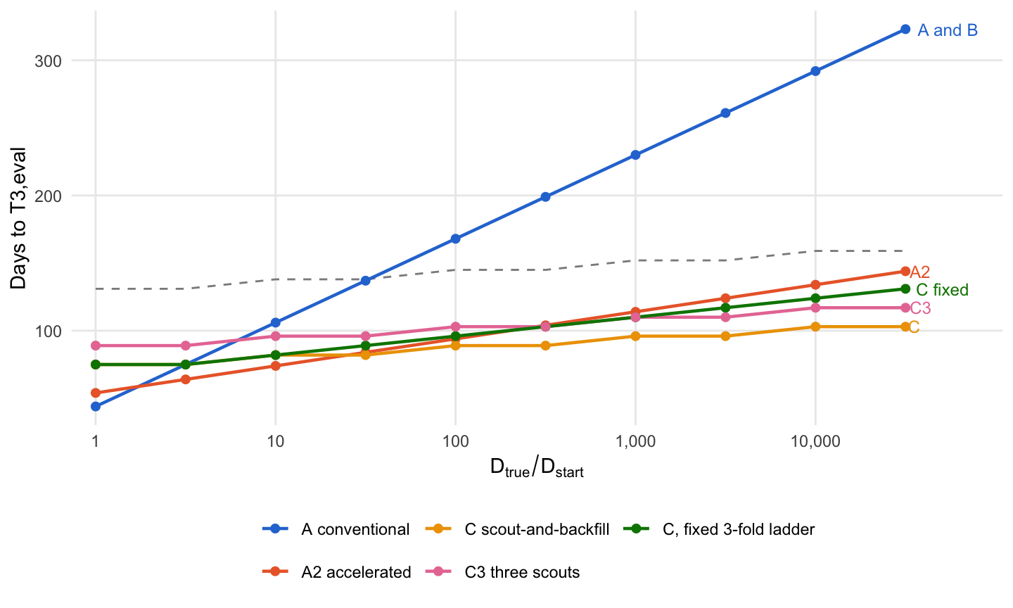
The time saving against A2 is arithmetic, and Section 4 shows it. Each half-log rung costs A2 a 3-day step-up plus a 7-day review, 10 days. The scout crosses two half-log rungs in a week while its FLC has not moved, 3.5 days a rung. The difference, 6.5 days a rung or 13 days a decade, is offset by a confirmation penalty of about seven weeks that A2 mostly avoids. Spec §15 made A2’s review window 7 days “fast on purpose”. At 14 days, the saving clears eight weeks from a gap of about 3,200-fold (Section 8). That window decides the time verdict, and it is a protocol fact the simulation cannot supply.
The scout overshoots, which Spec §7 did not expect. The scout’s ladder stops two half-log steps above the true active dose, 10-fold, in the base case and at every gap. Its backfill patients then confirm on the first attempt at that dose. Spec §7 predicted the opposite, a nomination below the active dose and backfill cohorts that fail to confirm. The reason is a mismatch of time windows: the active dose is calibrated on four weeks of exposure (Spec §10), and the scout is read five days after each rung. Section 6 has the detail.
Recommendation. ⚠️ Do not build Phase 2 yet. Settle two things first, both cheaper than the next phase:
Find the single-patient review window that real accelerated TCE protocols use, since it moves the time verdict across the contour.
Decide how the backfill dose is nominated, given that the scout overshoots.
Section 11 sets out the reasoning, Section 10 lists 14 places where the specification needed a decision it did not make, and Section 12 picks out the six choices made here that could change the answer.
Out of scope here, stated once.
❌ Variability of any kind: no inter-individual variability, no stochastic enrolment, no assay noise. Every result is a single deterministic value (Phases 2 and 4).
❌ Toxicity: no cytokine release syndrome (CRS), immune effector cell-associated neurotoxicity syndrome (ICANS) or neutropenia, and every safety gate passes (Phase 3). Simon’s toxicity trigger for ending A2’s accelerated phase cannot fire, so A2 runs the FLC-movement trigger only.
❌ Two step-up doses, serial and rolling second scouts, the first-dose limit \(F_{\rm start}\), renal confounding and Archetype 3. C3, three scouts climbing together, is the only multi-scout design run.
1. What Was Built
The model is Spec §8 and §9 as written, with FLC kept as an algebraic function of plasma-cell mass. Subcutaneous first-order absorption into a two-compartment model with linear clearance drives a plasma-cell turnover model. The drug’s kill rate is \(k_{\max} C^h/(EC_{50}^h + C^h)\), and FLC is \(L/L_0 = (1-f_{\rm res})P + f_{\rm res}\). Because the PK is linear and \(EC_{50}\) is solved for each scenario (Spec §10), every dose can be written as a multiple of \(D_{\rm true}\). One calibration then serves every scenario, and a scenario is fully described by how many grid steps \(D_{\rm true}\) sits above \(D_{\rm start}\).
The trial engine steps through events in calendar time. It is driven by three things. Each patient’s FLC trajectory comes from their own dose history. Weekly FLC samples have results available \(T_{\rm PD,ready}\) days later. Recruitment delivers one patient every \(7/\lambda\) days to whichever unit is recruiting. A conventional patient continues weekly target dosing after the step-up, and is followed until the design’s own \(T_{3,\rm eval}\).
Every input to the base case, and where it came from. “My call” marks a value the specification did not settle
Last confirming patient’s first dose + \(W_{\rm full}\) + \(T_{\rm PD,ready}\)
My call: the day-28 result is needed to count
Next level opens (3-patient cohort)
Last patient’s target dose (day 3) + \(W_{\rm cohort}\)
Spec §15
Accelerated phase in A2 ends
First FLC result below \(\theta_{\rm move}\) in any patient; the highest level dosed expands to 3 patients
Spec §6 PD variant; expanding the current level is Simon’s rule
Catch-up in B
Up one level a week, to the highest level whose review is complete
Spec §6
Scout stop to backfill opening
7 d
My call: Spec §20 mentions a review lag with no value
Recruitment
\(\lambda = 1\) a week; a unit recruits from the time the previous unit filled, and arrivals wait for it to open
My call: Spec §20 says the conventional arm “has been enrolling throughout”
Backfill recruitment
Reactive: starts when the scout stops
Spec §20
Observation after a dose
48 h after any dose higher than every earlier dose for that patient
My call: Spec §19 has no value
Administrative cap
16 grid steps, \(10^8 D_{\rm start}\)
My call
The prediction-error grid collapses to one axis in Phase 1. No design rule reads \(D_{\rm pred}\), so \(R_{\rm predicted-gap}\) and \(E_{\rm pred}\) enter only through their product \(D_{\rm true}/D_{\rm start}\). The 18 cells of Spec §12 map onto 10 values of the gap, from 1 to \(10^{4.5}\), in half-log steps; Spec’s \(E_{\rm pred}\) of 3 and 30 become \(10^{0.5}\) and \(10^{1.5}\). Section 5 shows the 18 cells. Section 10 records this as a problem with the specification.
2. Calibration
FLC on day 28 and the day FLC first falls below 10%, by target dose
cal <-tibble(offset =-3:3) %>%mutate(`Target dose / D_true`=signif(10^(offset /2), 2),`L/L0, day 7`=round(ctx$tab[8, as.character(offset)], 3),`L/L0, day 28`=round(ctx$tab[29, as.character(offset)], 3),`First day below 0.10 on weekly dosing`=map_dbl(offset, ~ { w <-which(ctx$tab[, as.character(.x)] <0.1); if (length(w)) w[1] -1elseNA }))h1 <-calibrate(modifyList(bio_base, list(h =1)))kable(cal %>%select(-offset), align ="rrrr",caption ="The conventional regimen at each grid level around D_true, in the reference patient")
The conventional regimen at each grid level around D_true, in the reference patient
Target dose / D_true
L/L0, day 7
L/L0, day 28
First day below 0.10 on weekly dosing
0.032
0.998
0.955
NA
0.100
0.990
0.774
NA
0.320
0.946
0.285
99
1.000
0.750
0.050
19
3.200
0.319
0.034
11
10.000
0.084
0.032
7
32.000
0.041
0.031
5
The calibration of Spec §10 holds with \(h = 1.5\): the regimen at \(D_{\rm true}\) gives \(L/L_0 = 0.05\) on day 28, and one grid step lower gives 0.285, above the 0.20 margin. With \(h = 1\) the step below gives 0.132 and fails the margin, so the half-log grid is too fine to separate adjacent levels at \(h = 1\).
The active dose is active only on the 28-day clock. A patient kept on the regimen one grid step below \(D_{\rm true}\) reaches profound suppression on day 99. Spec §10 defines the active dose at the PD assessment, and the engine keeps to that, but on continued weekly dosing the step below is active too, just later. A conventional design that waited longer would confirm a lower dose.
One week at a dose says little about it. The day-7 column is what a scout sees after one rung. At \(D_{\rm true}\), FLC has fallen only to 0.75; profound suppression within a week needs a dose 10-fold higher. This is the mechanism behind the overshoot in Section 6.
3. One Scenario Walked Through
Run the three main designs at a gap of 100-fold and draw every patient
m_ex <-4runs_ex <-map(c(A ="A", A2 ="A2", C ="C"), ~ designs[[.x]](m_ex, trial_base, ctx))swim <-imap_dfr(runs_ex, function(r, d) {map_dfr(seq_along(r$pts), function(i) { pt <- r$pts[[i]]if (pt$t1 > r$T3) return(NULL) days <-0:floor(r$T3 - pt$t1) L <-patient_L(pt, ctx)[days +1] lev <-approx(pt$doses$time, pt$levels, xout = days, method ="constant", rule =2)$ytibble(design = d, id = i, day = pt$t1 + days, L = L, level = lev, role = pt$role) })}) %>%mutate(status =factor(case_when(L <0.1~"Suppressed", L <0.7~"Moved", TRUE~"Not moved"),levels =names(status_cols)),design =factor(design_names[design], levels = design_names[c("A", "A2", "C")]))
Code
lab <- swim %>%group_by(design, id) %>%summarise(day =min(day), level =if (first(role) =="scout") paste(first(level), "to", last(level)) elseas.character(first(level)),.groups ="drop")ggplot(swim, aes(day, factor(-id))) +geom_tile(aes(fill = status), height =0.7, width =1) +geom_text(data = lab, aes(label = level), hjust =1.4, size =2.8, colour ="grey30") +facet_grid(design ~ ., scales ="free_y", space ="free_y") +scale_fill_manual(values = status_cols, name ="FLC") +labs(x ="Days from the first dose in the study", y =NULL) +theme(axis.text.y =element_blank(), panel.grid.major.y =element_blank(),strip.text.y =element_text(angle =0, hjust =0))
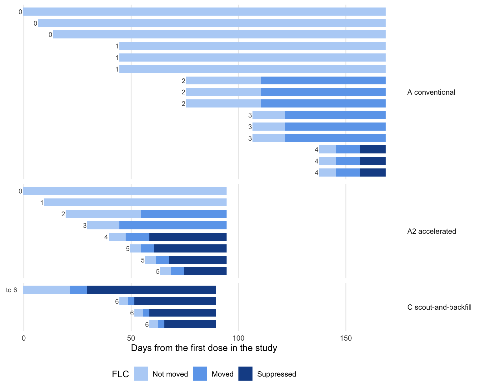
Figure 1: Every patient in Designs A, A2 and C when the true active dose is 100-fold above the starting dose (grid level 4), from their first dose to the design’s T3,eval. Each bar is one patient, its shade the FLC status that day, and the number at its left the target-dose grid level they received, with 4 the active dose. Under C, the top bar is the scout, who climbs from level 0 to level 6, and the three below are the backfill cohort.
Design A climbs one half-log level every 31 days. Each cohort fills while the previous cohort is under review, so a rung costs the 3 days to the last patient’s target dose plus the 28-day review. The first cohort has to wait for accrual of 3 patients, 14 days. Level 4 opens on day \(14 + 3 + 28 + 3 \times 31 = 138\), and its three patients finish evaluation 30 days later, on day 168.
Design A2 climbs one level every 10 days until a patient’s FLC moves. At this gap, movement first shows at a level above the active dose, which is expanded to three patients and confirmed there, one grid step too high. \(T_{3,\rm eval}\) is day 94.
Design C’s scout climbs and stops on the dates in the table below. The scout stops on day 38. Backfill opens 7 days later, recruits 3 patients a week apart, and the last completes evaluation on day 89.
The scout’s decisions
runs_ex$C$log %>%mutate(`Dose / D_true`=signif(10^((level - m_ex) /2), 2), L =round(L, 3),Decision =case_when(step ==0~"Stop: nominate this dose", step ==2~"Not moved: up 10-fold",TRUE~"Moved: up 3.16-fold")) %>%select(`Rung dosed (day)`= dose_day, `Grid level`= level, `Dose / D_true`,`FLC sampled (day)`= sample_day, `L/L0`= L, `Result and decision (day)`= result_day, Decision) %>%kable(align ="rrrrrrl", caption ="The scout's ladder at a gap of 100-fold. Grid level 4 is D_true")
The scout’s ladder at a gap of 100-fold. Grid level 4 is D_true
Rung dosed (day)
Grid level
Dose / D_true
FLC sampled (day)
L/L0
Result and decision (day)
Decision
3
0
0.01
8
1.000
10
Not moved: up 10-fold
10
2
0.10
15
0.987
17
Not moved: up 10-fold
17
4
1.00
22
0.691
24
Moved: up 3.16-fold
24
5
3.20
29
0.112
31
Moved: up 3.16-fold
31
6
10.00
36
0.034
38
Stop: nominate this dose
The scout passes the active dose and keeps going. On the rung at \(D_{\rm true}\), the day-5 sample reads just under 0.70, so the brake engages. The next rung, 3.16-fold above \(D_{\rm true}\), reads just above 0.10. Only the rung 10-fold above \(D_{\rm true}\) stops it, and that becomes the nominated dose \(D^*\). Two of these readings sit within 0.02 of a threshold, so the ladder is sensitive to small changes in any input, as Section 8 shows.
Figure 2: T3,eval, the days from the first dose until 3 patients have completed evaluation on a confirmed regimen, against the gap between the starting dose and the true active dose. Design B is not drawn: catch-up does not change when levels open, so its T3,eval equals Design A’s at every gap. The dashed line marks Design C’s T3,eval plus eight weeks: a design above it is slower than C by more than the Spec §1 contour.
The same numbers as a table
base %>%select(m, design, T3) %>%pivot_wider(names_from = design, values_from = T3) %>%mutate(`D_true / D_start`=format(signif(10^(m /2), 2), big.mark =","), `A − C`= A - C, `A2 − C`= A2 - C) %>%select(`D_true / D_start`, A, A2, B, C, C_fixed, C3, `A − C`, `A2 − C`) %>%kable(caption ="T3,eval in days for each design, and the time Design C saves against A and A2")
T3,eval in days for each design, and the time Design C saves against A and A2
D_true / D_start
A
A2
B
C
C_fixed
C3
A − C
A2 − C
1.0
44
54
44
75
75
89
-31
-21
3.2
75
64
75
75
75
89
0
-11
10.0
106
74
106
82
82
96
24
-8
32.0
137
84
137
82
89
96
55
2
100.0
168
94
168
89
96
103
79
5
320.0
199
104
199
89
103
103
110
15
1,000.0
230
114
230
96
110
110
134
18
3,200.0
261
124
261
96
117
110
165
28
10,000.0
292
134
292
103
124
117
189
31
32,000.0
323
144
323
103
131
117
220
41
Every curve is a straight line in the log of the gap, so the comparison reduces to cost per rung.
Cost of a half-log rung of the gap, base case
Design
Days per half-log rung
Where it comes from
A
31
3 days to the target dose + 28-day review
A2
10
3 days to the target dose + 7-day review, until FLC moves
C
3.5
7 days for two rungs while FLC has not moved
C, fixed ladder
7
7 days a rung
The intercepts are set by the confirmation penalty. Design C’s \(T_{3,\rm eval} - T_{\rm FLC}\) is 51 days at every gap: 7 days of review, 14 days to recruit the second and third backfill patients, and 30 days of evaluation. Design A’s is 7 days at every gap above the first, because the confirming cohort is the one that first showed suppression. This penalty is what hypothesis 4 of Spec §26 predicted. It also explains why C loses to A2 at gaps up to 10-fold: A2 has not yet had enough rungs to fall behind by the difference in confirmation penalties.
C3, three scouts climbing together, costs 14 days over C at one patient a week, the time to recruit two more scouts before the ladder starts, and nothing with no accrual wait (Section 8).
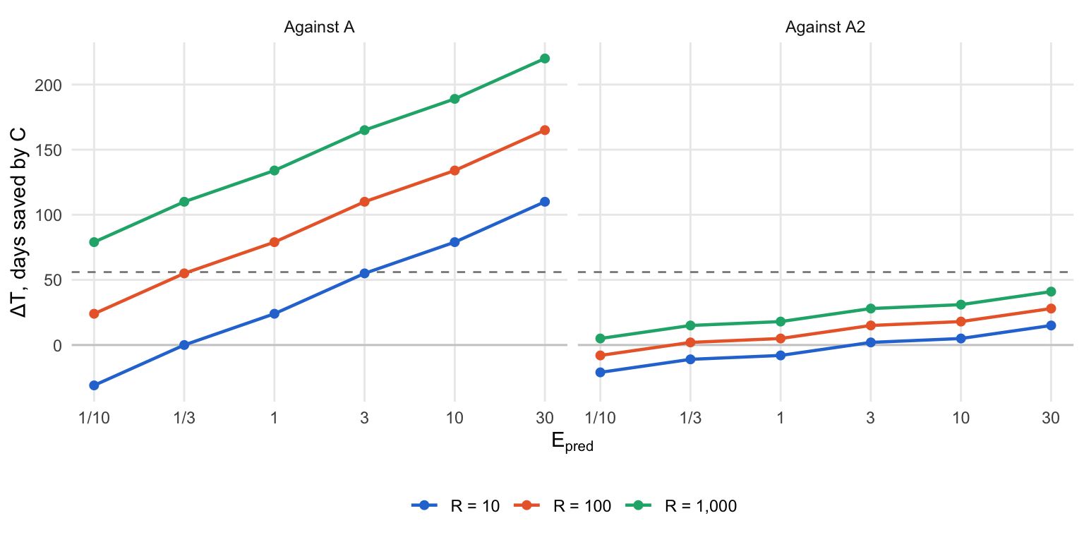
Figure 3: Days saved by Design C, ΔT, against the prediction error E_pred = D_true / D_pred, for three predicted gaps R = D_pred / D_start, against Design A (left) and Design A2 (right). The dashed line is the eight-week contour of Spec §1. Each line is the same curve shifted, since only the product R × E_pred enters Phase 1.
A well-predicted active dose removes the benefit against A2, as Spec §26 hypothesis 2 says. With \(E_{\rm pred} = 1\), Design C saves at most 18 days against A2 at any of the three predicted gaps. Against A, most of the saving comes from the predicted gap \(R\): at \(E_{\rm pred} = 1\) the saving is 24 days when \(R = 10\) and 79 when \(R = 100\). The largest saving against A2 in the whole grid, 41 days, needs a predicted gap of 1,000 and an active dose 30-fold above the prediction.
6. Where the Scout’s Dose Lands
Nominated and confirmed dose relative to D_true
base %>%filter(design %in%c("A", "A2", "C", "C_fixed", "C3")) %>%group_by(Design = design_names[design]) %>%summarise(`Scout's D*, grid steps above D_true`=paste(sort(unique(D_star_vs_true)), collapse =", "),`Confirmed dose, grid steps above D_true`=paste(sort(unique(confirmed_vs_true)), collapse =", "),`Backfill cohorts needed`=paste(sort(unique(backfill_cohorts)), collapse =", "),`Patients dosed above D_true`=paste(unique(range(N_above)), collapse =" to ")) %>%mutate(across(everything(), ~na_if(.x, ""))) %>%kable(caption ="Dose selection across the 10 gaps. One grid step is 3.16-fold; NA where the design has no scout or no backfill")
Dose selection across the 10 gaps. One grid step is 3.16-fold; NA where the design has no scout or no backfill
Design
Scout’s D*, grid steps above D_true
Confirmed dose, grid steps above D_true
Backfill cohorts needed
Patients dosed above D_true
A conventional
NA
0
NA
0
A2 accelerated
NA
1
NA
3
C scout-and-backfill
2
2
1
4
C, fixed 3-fold ladder
1, 2
1, 2
1
4
C3 three scouts
2
2
1
6
The PD-guided scout nominates a dose 10-fold above \(D_{\rm true}\) at every gap, and the fixed ladder one or two grid steps above. Backfill at \(D^*\) then confirms on the first cohort, so Spec §7’s non-confirmation cycles never occur, and Spec §4’s scoring puts the error where it said it would, in dose selection, outside \(T_{3,\rm eval}\). Four patients, the scout and three backfill patients, receive a dose above \(D_{\rm true}\). A2 confirms one step high, with three patients above \(D_{\rm true}\).
Spec §7 expected the nomination to sit low, because carried-over drug and carried-over depletion push the scout’s FLC down early. Both effects are present, and a larger one runs the other way. The calibration defines \(D_{\rm true}\) by 28 days of exposure, while the scout spends 7 days on each rung and is read on day 5. The table in Section 2 shows what follows: a week at \(D_{\rm true}\) leaves FLC at 0.75, and only a dose near 10-fold higher suppresses within a week. The scout stops at the first dose that suppresses within one rung. That dose is set by \(k_{\max}\) and the sampling day, and the 28-day active dose does not enter.
Nominating below \(D^*\) recovers the dose at no cost in time, here. Nominating \(D^*/10\) puts the backfill on \(D_{\rm true}\), which confirms, and \(T_{3,\rm eval}\) is unchanged (Section 8). Nominating \(D^*/30\) fails once and costs one conventional rung. The rule only works because the overshoot is a constant two steps in this deterministic model. Phase 4, with variability between patients, is where a fixed downward offset would be tested.
7. Patients and Workload
Patient and workload counters at gaps of 100 and 30,000-fold
base %>%filter(m %in%c(4, 9)) %>%transmute(`D_true / D_start`=format(signif(10^(m /2), 2), big.mark =","), Design = design_names[design],`Patients`= N, `N_sub`= N_sub, `Patient-weeks unsuppressed`=round(N_pw),`Patient-weeks at ≤ D_true/10`=round(N_pw_low),`Administrations`= admins, `Observation, patient-hours`= H_obs,`Most hours for one patient`= H_obs_max_pt) %>%kable(caption ="Counters up to each design's own T3,eval. N_sub is the number of patients whose highest target dose was below D_true")
Counters up to each design’s own T3,eval. N_sub is the number of patients whose highest target dose was below D_true
D_true / D_start
Design
Patients
N_sub
Patient-weeks unsuppressed
Patient-weeks at ≤ D_true/10
Administrations
Observation, patient-hours
Most hours for one patient
100
A conventional
15
12
197
162
216
1440
96
100
A2 accelerated
8
4
53
36
77
768
96
100
B catch-up
15
12
197
127
216
2304
240
100
C scout-and-backfill
4
0
7
2
32
576
288
100
C, fixed 3-fold ladder
4
0
11
3
33
624
336
100
C3 three scouts
6
0
16
7
60
1152
288
32,000
A conventional
30
27
729
694
762
2880
96
32,000
A2 accelerated
13
9
142
126
171
1248
96
32,000
B catch-up
30
27
729
598
762
8064
480
32,000
C scout-and-backfill
4
0
10
4
34
672
384
32,000
C, fixed 3-fold ladder
4
0
16
8
38
864
576
32,000
C3 three scouts
6
0
23
13
66
1440
384
The patient saving is large against both comparators and does not depend on the comparator’s review window. Design C’s \(N_{\rm sub}\) is zero at every gap, since the scout always climbs past \(D_{\rm true}\) and the backfill starts at or above it. Patient-weeks with FLC at or above 10% of baseline, \(N_{\rm pw}\), are 7 to 15 times fewer than under A2 at the two gaps in the table, and 27 to 76 times fewer than under A.
Catch-up (Design B) moves only the low-dose counter. Its patients move only to levels whose review is complete, one behind the level open, so they reach \(D_{\rm true}/3.16\) shortly before the trial confirms and never suppress inside \(T_{3,\rm eval}\). \(N_{\rm sub}\) and \(N_{\rm pw}\) are unchanged from A; patient-weeks at a dose 10-fold or more below \(D_{\rm true}\) fall by 14% to 22%. That last counter is my addition, since Spec §6’s “patient-time at clearly subactive doses” had no definition.
Workload runs in opposite directions per patient and per trial, as Spec §1 predicted. The scout carries 6 to 8 dose increases, each with 48 hours of observation, against 2 for a conventional patient. Across the trial, C needs fewer observation hours than A or A2 because it treats half as many patients as A2, or fewer. Extra clinic visits, \(N_{\rm visit}\), are not computed: they need a standard schedule to subtract, which Spec §19 does not define.
8. Sensitivity Analyses
One-at-a-time sensitivities from Spec §21, plus three combinations
sens <-list(list("Base case", list(), list()),list("Enrolment 0.5 a week", list(lam =0.5), list()),list("Enrolment 2 a week", list(lam =2), list()),list("No accrual wait", list(lam =Inf), list()),list("A2 review window 14 d", list(W_cohort1 =14), list()),list("3-patient review window 14 d", list(W_cohort3 =14), list()),list("3-patient review window 21 d", list(W_cohort3 =21), list()),list("PD turnaround 1 d", list(T_PD =1), list()),list("PD turnaround 3 d", list(T_PD =3), list()),list("PD turnaround 5 d", list(T_PD =5), list()),list("Scout step every 14 d", list(step_days =14), list()),list("Anticipatory backfill", list(backfill ="anticipatory"), list()),list("Stop-to-backfill lag 0 d", list(review_lag =0), list()),list("Stop-to-backfill lag 14 d", list(review_lag =14), list()),list("Nominate D*/30", list(nominate_offset =-3), list()),list("Nominate D*/10", list(nominate_offset =-2), list()),list("Nominate 3.16 D*", list(nominate_offset =1), list()),list("θ_move 0.50", list(theta_move =0.5), list()),list("θ_move 0.85", list(theta_move =0.85), list()),list("F_quiet 3.16", list(q_steps =1), list()),list("F_quiet 31.6", list(q_steps =3), list()),list("θ_stop 0.25", list(theta_stop =0.25), list()),list("W_full 14 d", list(W_full =14), list()),list("Plasma-cell half-life 30 d", list(), list(t_half_P =30)),list("Plasma-cell half-life 180 d", list(), list(t_half_P =180)),list("Hill h = 1", list(), list(h =1)),list("Hill h = 2", list(), list(h =2)),list("k_max 0.5 per day", list(), list(kmax =0.5)),list("k_max 3 per day", list(), list(kmax =3)),list("Combined: A2 review 14 d, anticipatory backfill", list(W_cohort1 =14, backfill ="anticipatory"), list()),list("Combined: F_quiet 31.6, anticipatory backfill", list(q_steps =3, backfill ="anticipatory"), list()),list("Combined: enrolment 0.5 a week, anticipatory backfill", list(lam =0.5, backfill ="anticipatory"), list()))ms_s <-c(4, 6, 9)sens_out <-map_dfr(sens, function(s) { tb <-modifyList(trial_base, s[[2]]) cx <-if (length(s[[3]]) ||!is.null(s[[2]]$W_full)) make_ctx(modifyList(bio_base, s[[3]]), tb) else ctxrun_grid(ms_s, c("A", "A2", "C"), tb, cx) %>%mutate(scenario = s[[1]])})mark <-function(x) ifelse(x >= contour, paste0("✅ ", x), as.character(x))sens_out %>%select(scenario, m, design, T3, D_star_vs_true, confirmed_vs_true) %>%pivot_wider(names_from = design, values_from =c(T3, D_star_vs_true, confirmed_vs_true)) %>%mutate(dA = T3_A - T3_C, dA2 = T3_A2 - T3_C) %>%group_by(scenario) %>%summarise(`vs A, 100×`=mark(dA[m ==4]), `vs A, 1,000×`=mark(dA[m ==6]), `vs A, 30,000×`=mark(dA[m ==9]),`vs A2, 100×`=mark(dA2[m ==4]), `vs A2, 1,000×`=mark(dA2[m ==6]), `vs A2, 30,000×`=mark(dA2[m ==9]),`C confirms at`=paste(unique(confirmed_vs_true_C), collapse =", ")) %>%slice(match(map_chr(sens, 1), scenario)) %>%rename(Scenario = scenario) %>%kable(align ="lrrrrrrr",caption ="Days saved by Design C at three gaps (100, 1,000 and about 30,000-fold); ✅ marks a saving of eight weeks or more. The last column is the grid step, above D_true, at which C's backfill confirms")
Days saved by Design C at three gaps (100, 1,000 and about 30,000-fold); ✅ marks a saving of eight weeks or more. The last column is the grid step, above D_true, at which C’s backfill confirms
Scenario
vs A, 100×
vs A, 1,000×
vs A, 30,000×
vs A2, 100×
vs A2, 1,000×
vs A2, 30,000×
C confirms at
Base case
✅ 79
✅ 134
✅ 220
5
18
41
2
Enrolment 0.5 a week
✅ 116
✅ 193
✅ 312
4
25
✅ 60
2
Enrolment 2 a week
✅ 82.5
✅ 137.5
✅ 223.5
8.5
21.5
44.5
2
No accrual wait
✅ 79
✅ 134
✅ 220
8
21
44
2
A2 review window 14 d
✅ 79
✅ 134
✅ 220
23
50
✅ 94
2
3-patient review window 14 d
39
✅ 74
✅ 130
5
18
41
2
3-patient review window 21 d
51
✅ 92
✅ 157
5
18
41
2
PD turnaround 1 d
✅ 86
✅ 141
✅ 220
12
25
41
1, 2
PD turnaround 3 d
✅ 86
✅ 141
✅ 220
12
25
41
2
PD turnaround 5 d
✅ 79
✅ 134
✅ 220
5
18
41
3, 2
Scout step every 14 d
✅ 58
✅ 106
✅ 185
-16
-10
6
1
Anticipatory backfill
✅ 93
✅ 148
✅ 234
19
32
55
2
Stop-to-backfill lag 0 d
✅ 79
✅ 134
✅ 220
5
18
41
2
Stop-to-backfill lag 14 d
✅ 79
✅ 134
✅ 220
5
18
41
2
Nominate D*/30
48
✅ 103
✅ 189
-26
-13
10
0
Nominate D*/10
✅ 79
✅ 134
✅ 220
5
18
41
0
Nominate 3.16 D*
✅ 79
✅ 134
✅ 220
5
18
41
3
θ_move 0.50
✅ 86
✅ 141
✅ 220
12
25
41
2
θ_move 0.85
✅ 79
✅ 134
✅ 220
-5
8
31
2
F_quiet 3.16
✅ 72
✅ 120
✅ 192
-2
4
13
1
F_quiet 31.6
✅ 93
✅ 148
✅ 234
19
32
55
2, 3
θ_stop 0.25
✅ 86
✅ 141
✅ 227
12
25
48
1
W_full 14 d
✅ 86
✅ 141
✅ 227
2
15
38
1
Plasma-cell half-life 30 d
55
✅ 110
✅ 196
2
15
38
1
Plasma-cell half-life 180 d
✅ 86
✅ 141
✅ 220
12
25
41
2
Hill h = 1
✅ 86
✅ 141
✅ 220
2
15
31
1, 2
Hill h = 2
✅ 86
✅ 141
✅ 220
12
25
41
2
k_max 0.5 per day
✅ 86
✅ 141
✅ 220
2
15
31
1, 2
k_max 3 per day
✅ 86
✅ 141
✅ 220
12
25
41
2
Combined: A2 review 14 d, anticipatory backfill
✅ 93
✅ 148
✅ 234
37
✅ 64
✅ 108
2
Combined: F_quiet 31.6, anticipatory backfill
✅ 107
✅ 162
✅ 248
33
46
✅ 69
2, 3
Combined: enrolment 0.5 a week, anticipatory backfill
✅ 151
✅ 228
✅ 347
39
✅ 60
✅ 95
2
Two rows not in the table could not be run as specified.\(f_{\rm res} = 0.05\), a Spec §9 sensitivity, fails Spec §10’s own condition \(f_{\rm res} < 0.05\), so no dose can be calibrated. \(\theta_{\rm stop} = 0.05\), a Spec §13 sensitivity, puts the stop threshold on the calibration target of 0.05, the boundary case Spec §10 was written to avoid. For hypothesis 20 the analytic bound is enough: the lowest FLC any dose can reach is \(f_{\rm res} + (1 - f_{\rm res})\,k_{\rm out}/(k_{\rm out} + k_{\max})\), about \(f_{\rm res} + 0.011\). The stop can fire only below \(f_{\rm res} \approx 0.089\), and the calibration only below 0.05.
Three levers change the time verdict against A2:
The A2 review window. At 14 days, C saves eight weeks or more from a gap of about 3,200-fold.
Anticipatory backfill, which removes 14 days of the confirmation penalty.
A larger quiet step, \(F_{\rm quiet} = 31.6\).
Combined, the last two clear eight weeks against A2 at the far end of the grid. Slow enrolment helps C against both comparators, because three-patient cohorts wait on accrual and the scout does not.
The scout’s own parameters move \(\Delta T\) by a week at a time.\(T_{\rm PD,ready}\), \(\theta_{\rm move}\), \(h\) and \(k_{\max}\) change the ladder by one rung in either direction. A later FLC sample misses the brake, takes a 10-fold step instead of 3.16, stops a week sooner and nominates one step higher, so a slower assay can make C faster. That is Spec §13’s missed brake. Hypothesis 5, that fast turnaround strongly raises the value of IPDE, does not hold here: turnaround trades a week of time against a grid step of overshoot.
The stop-to-backfill review lag changes nothing between 0 and 14 days, because the backfill is waiting on recruitment for longer than that. Its effect would appear only with anticipatory pre-screening.
9. The Hypotheses of Spec §26
Numbers quoted in the table below
fast <-run_grid(c(4, 9), c("A", "A2", "C", "C3"), modifyList(trial_base, list(lam =Inf)), ctx)g <-function(d, mm, col, df = base) df[[col]][df$design == d & df$m == mm]
Verdicts on the 21 hypotheses. ✅ supported, ❌ contradicted, ⚠️ partly, — not testable in Phase 1
#
Hypothesis
Verdict in Phase 1
1
Big gap, big gain
✅ Against A. ⚠️ Against A2 the gain grows with the gap but stays under eight weeks
2
Good prediction removes the benefit
✅ Against A2: at \(E_{\rm pred} = 1\) the saving is under three weeks for every \(R\). ⚠️ Against A the saving at \(E_{\rm pred} = 1\) is material once \(R \ge 100\)
3
Catch-up helps patients, not time
⚠️ Time unchanged by construction. The patient help is small: only patient-weeks at ≤ \(D_{\rm true}/10\) fall, from 694 to 598 at the largest gap
4
Backfill shrinks the gain
✅ The confirmation penalty is 51 days, against 7 for A
5
Fast PD turnaround raises the value
❌ Turnaround moves the ladder by a rung either way and trades time against overshoot
6
Operational burden is small when visits are scheduled anyway
— \(N_{\rm visit}\) needs a standard schedule Spec does not give. Per patient the scout carries 3 to 4 times the observation hours of a conventional patient
7
Escalation can outrun safety information
— No toxicity in Phase 1
8
ICANS stays unquantified
— Not modelled, by design
9
Fixed-ratio backfill undershoots
❌ It overshoots by two grid steps, and backfill never fails to confirm (Section 6)
10
At slow accrual, enrolment dominates the confirmation penalty
✅ The penalty is mostly recruitment and evaluation; the review lag is hidden under recruitment, and anticipatory backfill removes 14 days
11
Priming does not rescue acute safety
— No toxicity in Phase 1
12
A second scout repeats the first ladder
— Serial scouts not run
13
Most of the low-dose saving is the micro-cohort
✅ Of the 220 days C saves against A at the largest gap, A2 already saves 179; \(N_{\rm sub}\) falls from 27 (A) to 9 (A2) to 0 (C)
14
Rolling scouts are cheap in time, expensive in exposure
— Rolling scouts not run
15
PD-guided beats a fixed ladder
⚠️ Faster: 103 against 131 days at the largest gap. But it nominates one step higher, further from \(D_{\rm true}\)
16
Under fast accrual, cohort size moves patients, not time
❌ With no accrual wait, A2 still reaches \(T_{3,\rm eval}\) in 133 days against A’s 309. The difference comes from the review windows Spec §15 attaches to each cohort size, 7 days against 28
17
FLC turnaround shrinks the turnaround lever
✅ Consistent with 5: the lever moves the result by about a rung
18
The nomination sits lower than in the B-cell design
❌ in direction: the nomination sits above \(D_{\rm true}\). The B-cell design was not run
19
Renal confounding delays the stop
— Not run
20
The floor decides whether the design works
⚠️ Located analytically: the stop can fire only below \(f_{\rm res} \approx 0.089\), and calibration needs \(f_{\rm res} < 0.05\) (Section 8)
21
Three scouts keep the time saving and lose most of the patient saving
⚠️ Time kept: C3 matches C with no accrual wait. Patient saving also kept: \(N_{\rm sub}\) is 0 for C3, against 27 for A, because the scouts climb past \(D_{\rm true}\)
10. Problems Found in Specification 2
Each item is a place where building the engine needed a decision the specification did not make, or where two sections disagree. The decision taken here is in the table of Section 1.
\(D_{\rm pred}\) is read by no design rule, so Spec §12’s two ratios collapse into their product, and Figure 3 is Figure 2 re-indexed. Either drop \(E_{\rm pred}\) as a separate axis, or give a design a rule that uses the prediction. The natural candidate is A2’s step size or the length of its accelerated phase, which is how a team would use a prediction it trusted.
The conventional dose grid is not defined. Spec §13 gives the scout’s steps, and A, A2 and B need a grid too. A half-log grid was used for all designs.
“The prespecified PD assessment time” has no value. It sets the calibration and the confirmation rule. Day 28, the end of \(W_{\rm full}\), was used.
\(h\) is given as a range, and the low end fails Spec §10’s margin on a half-log grid (Section 2).
The active dose depends on the assessment time. On continued weekly dosing the level below \(D_{\rm true}\) also suppresses, by day 99 (Section 2). Spec §10’s definition is internally consistent, but the “true” active dose is a property of the 28-day clock.
Spec §7’s prediction that the nomination sits low is reversed in this model (Section 6). The carryover argument in §7 leaves out the short time the scout spends on each rung.
Two sensitivity values sit on Spec §10’s boundaries:\(f_{\rm res} = 0.05\) and \(\theta_{\rm stop} = 0.05\) (Section 8).
Hypothesis 16 conflicts with Spec §15. It attributes A2’s speed to cohort size, but §15 gives single-patient cohorts a 7-day review window and three-patient cohorts 28 days, so in the engine the window does the work.
Catch-up cannot reduce \(N_{\rm sub}\) as defined, because patients only reach levels whose review is complete, one below the open level, so none reaches \(D_{\rm true}\) before \(T_{3,\rm eval}\). Hypothesis 3 needs a definition of “clearly subactive”; Section 7 uses 10-fold or more below \(D_{\rm true}\).
Spec §6 asks for Simon’s double dose steps in A2 and also for “everything else matches Design A”. The same grid was used, so that A against A2 isolates cohort size.
A2’s toxicity trigger cannot fire before Phase 3. Only the FLC-movement variant runs in Phase 1. Spec §6 also does not say which level expands when movement shows; the highest level dosed was used, as in Simon.
The recruitment model is unstated. Whether patients who arrive during a review window wait for the next cohort decides how much accrual the conventional arm hides. Here they wait, which favours the conventional designs.
The scout’s FLC sampling day is unstated. It sets which rung the brake and the stop fire on (Section 8); day \(7 - T_{\rm PD,ready}\) after each rung was used.
The workload counters need inputs Spec §19 does not give: observation hours per dose, and a standard visit schedule to subtract for \(N_{\rm visit}\).
11. Recommendation
ImportantRecommendation
⚠️ Do not build Phase 2 yet. Against Design A2, the comparator a clinical team would propose, scout-and-backfill saves at most 41 days, short of the eight-week contour everywhere on the prediction-error grid. It does treat no patient only at subactive doses. Settle three things before the next phase:
Find the single-patient review window that real accelerated TCE protocols use. At 7 days the time case fails; at 14 days it clears eight weeks from a gap of about 3,200-fold.
Decide how the backfill dose is nominated. The scout stops 10-fold above \(D_{\rm true}\), and the backfill patients inherit that dose.
Fold the 14 decisions in Section 10 back into Specification 2.
If the review window keeps the saving under eight weeks, stop at Phase 1 and take up the healthy volunteer route.
The time case fails against the realistic comparator. Against Design A2 it saves at most 41 days, short of the eight-week contour anywhere on the prediction-error grid, while treating no patient only at subactive doses. That is the third case of Spec §26b, “\(\Delta N_{\rm sub}\) material, \(\Delta T\) not”, which §26b calls a weaker argument for accepting an unquantified delayed-toxicity risk. Against Design A, the saving is material from a gap of about 100-fold.
Settle three things before building Phase 2. Phase 2 adds stochastic enrolment, sentinel staggering and operational counters. It will widen the numbers into bands without moving the arithmetic of Section 4, and that arithmetic is what decides the verdict.
Find A2’s real review window. The time verdict turns on whether a safety committee reviews a single-patient cohort in 7 days or 14. Published accelerated TCE escalations, including the GB261 protocol already on the references page, should say. If the answer is 14 days or more, the time case for IPDE is material from a gap of about 3,200-fold, and the project should continue on that axis.
Decide the nomination rule. The scout overshoots \(D_{\rm true}\) by 10-fold here, and the backfill patients inherit that dose. Two options:
Nominate below the scout’s stopping dose, as \(D^*/10\) does here at no cost in time.
Lengthen the time on each rung once FLC has moved.
Either changes Spec §7 and §13, and the choice should be made before variability makes it harder to see.
Resolve the 14 problems in Section 10, most of which are a sentence each, and fold the decisions taken here back into Specification 2.
If the review-window answer keeps the time case below eight weeks, consider stopping at Phase 1. Report the patient benefit and the overshoot, and take up the healthy volunteer route (tce-hv.qmd), which attacks the same gap without a within-patient ladder.
12. Choices That Could Change the Answer
WarningChoices made here that the specification did not settle
The full list is the table in Section 1, and every value there marked “My call” is one. These six are the ones whose alternatives move a result in this document.
The six choices whose alternatives would change a result
Choice
Value used
What changes if it is wrong
Review window for a single-patient cohort in A2
7 days, Spec §15’s base
At 14 days the saving against A2 clears eight weeks from a gap of about 3,200-fold, and the time verdict reverses (Section 8)
PD assessment time, for calibration and for confirming a dose
Day 28 after the first dose
Sets which dose counts as active; a later assessment makes a lower dose active (Section 2), a shorter one shrinks the overshoot (the \(W_{\rm full}\) = 14 d row of Section 8)
Scout’s FLC sample
Day \(7 - T_{\rm PD,ready}\) after each rung
Sets which rung the brake and the stop fire on, and so the overshoot, by one grid step either way (Section 8)
Hill coefficient \(h\)
1.5
At \(h = 1\) the calibration margin of Spec §10 fails; the saving against A2 falls by up to 10 days
Dose grid
Half-log for every design
Each design’s cost per rung (Section 4) is per half-log step; a finer grid for A and A2 slows them, a coarser one speeds them up
Recruitment
Arrivals during a review window wait for the next cohort
Favours A and A2. If they do not wait, three-patient cohorts pay accrual at every rung and the saving against A grows