library(dplyr)
library(ggplot2)
library(xgxr)

xgx_theme_set()
knitr::opts_chunk$set(fig.height = 4, fig.width = 5)Logistic Regression: Diagnostics
Checking calibration, residuals and linearity, and the gaps left in the checklist
PMX guide
working document
A minimal set of diagnostics for a logistic regression fit to dose-response data: calibration against observed rates, average residual versus outcome, and linearity of the continuous covariates.
Draft, with gaps. Section 5 lists what this page does not yet do: a Hosmer-Lemeshow test, an \(R^2\) calculation, and a Brier score, among others. What is here runs against real data.
1. Purpose
A logistic regression of dose against adverse event rate or overall response rate is a common analysis in dose finding. Given a fit, the next question is whether it is adequate. This page gives a minimal set of diagnostics for answering that.
Some of the original diagnostic work behind this page was developed by Edward Waldron and a summer intern.
2. The Data and the Fit
The same 96-patient synthetic dataset as Picking a Method; see the project index for the column list.
data <- readRDS("../../data/synthetic/dose-response/dose_tumor_resp.rds") |>
  mutate(observed = OR)

data |>
  group_by(DOSE) |>
  summarise(
    N = n(),
    N_responders = sum(OR == 1, na.rm = TRUE),
    Percent_responders = round(N_responders / N * 100)
  ) |>
knitr::kable(caption = "Response by dose")| DOSE | N | N_responders | Percent_responders |
|---|---|---|---|
| 1 | 2 | 0 | 0 |
| 2 | 1 | 0 | 0 |
| 4 | 1 | 1 | 100 |
| 6 | 3 | 1 | 33 |
| 8 | 14 | 9 | 64 |
| 10 | 9 | 7 | 78 |
| 12 | 10 | 7 | 70 |
| 14 | 5 | 5 | 100 |
| 16 | 51 | 37 | 73 |
model <- glm(OR ~ DOSE + ECOG0 + LD0, family = binomial, data = data)
f_trans <- function(x) exp(x) / (1 + exp(x))
3. Check Calibration: Observed Versus Predicted Probability
This compares the observed and predicted probability of response within ten bins of predicted probability. If the identity line (slope 1, intercept 0) passes through most of the intervals’ confidence bars, the fit’s calibration looks reasonable.
data_pred <- data |>
  mutate(
    pred = f_trans(predict(model)),
    group_id = Hmisc::cut2(pred, g = 10)
  )

data_plot <- data_pred |>
  group_by(group_id) |>
  summarise(
    total = n(),
    num_observed = sum(observed),
    mean_pred = mean(pred),
    mean_observed = mean(observed),
    upper_CI = binom::binom.confint(num_observed, total, conf.level = 0.95, method = "exact")$upper,
    lower_CI = binom::binom.confint(num_observed, total, conf.level = 0.95, method = "exact")$lower
  )

ggplot(data_plot, aes(x = mean_pred, y = mean_observed)) +
  geom_point() +
  geom_abline(slope = 1, intercept = 0, color = "blue") +
  geom_errorbar(aes(ymin = lower_CI, ymax = upper_CI), width = 0.005) +
  labs(x = "Predicted event rate", y = "Observed event rate")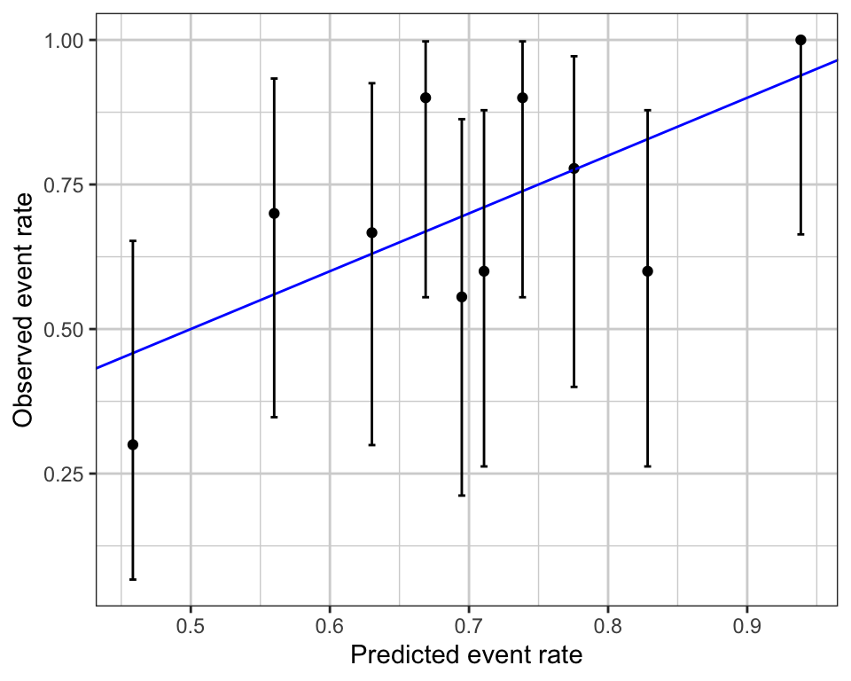
A formal companion to this plot is the Hosmer-Lemeshow test, not yet implemented here; see Open questions.
4. Check for Inadequacies: Average Residual Versus Outcome
The data is divided into bins by fitted value, with roughly equal patients per bin, and the average residual is plotted against the average fitted value for each bin. More bins show more local pattern in the residuals but each needs enough points to keep the average from being noisy. About 95% of binned residuals are expected to fall within \(\pm 2\) standard errors, i.e. \(\pm 2\sqrt{p(1-p)/n}\) for \(n\) points per bin.
n <- nrow(data)
nbins <- if (n >= 100) floor(sqrt(n)) else if (n > 10) 10 else floor(n / 2)

resid_bin <- data.frame(
  pred  = predict(model, type = "response"),
  resid = residuals(model)
) |>
  mutate(group_id = Hmisc::cut2(pred, g = nbins)) |>
  group_by(group_id) |>
  summarise(
    pred_mean  = mean(pred),
    resid_mean = mean(resid),
    resid_sd   = sd(resid),
    n          = length(pred),
    resid_upper =  1.96 * resid_sd / sqrt(n),
    resid_lower = -1.96 * resid_sd / sqrt(n)
  )

ggplot(resid_bin, aes(x = pred_mean, y = resid_mean)) +
  geom_point() +
  geom_ribbon(aes(ymin = resid_lower, ymax = resid_upper), alpha = 0.2) +
  geom_hline(yintercept = 0, color = "blue") +
  labs(x = "Average predicted response", y = "Average residual") +
  ggtitle(paste0("Average of ", signif(mean(resid_bin$n), 2), " data points per bin"))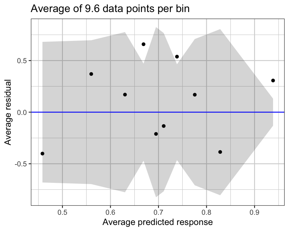
5. Check the Linearity Assumption on Continuous Covariates
Logistic regression assumes a linear relationship between each continuous covariate and the log-odds (logit) of the outcome. Plotting the logit against each covariate, with a loess smooth, checks that visually.
data |>
  mutate(logit = predict(model)) |>
  tidyr::pivot_longer(cols = c(DOSE, LD0)) |>
  ggplot(aes(x = value, y = logit)) +
  geom_point() +
  geom_smooth(method = "loess") +
  facet_wrap(~name, scales = "free_x") +
  labs(x = "Predictor", y = "Logit")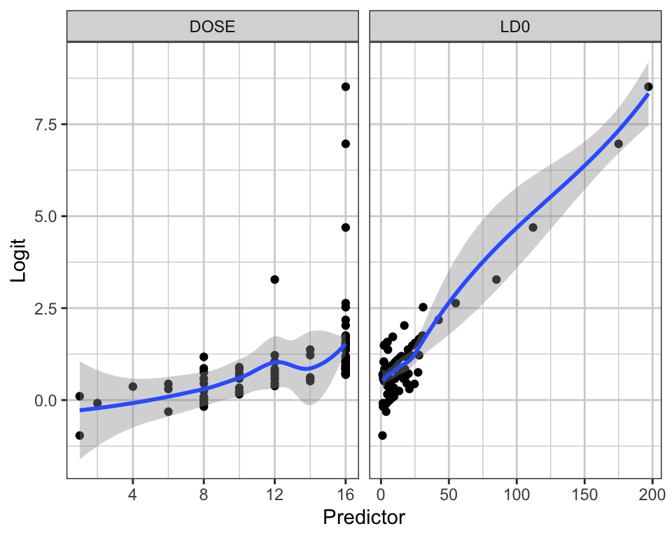
6. Open Questions
Carried over from the original working notes, unresolved:
- Hosmer-Lemeshow test. Not implemented.
glmtoolbox::hltestruns it, though that package may not be available in every R environment. - An \(R^2\) measure. Several candidates exist; see Frank Harrell’s discussion. The
rmspackage’sR2Measuresfunction gives a choice of which to use. - Brier score, covering both calibration and discrimination.
- Other metrics proposed in Harrell’s lecture notes on binary logistic regression, Section 8-40.
- The residual standard error used in the Section 4 plot should be reviewed against a reference rather than taken as given.